Here we show how to obtain venous DYNA CT and do fusions between arterial and venous datasets
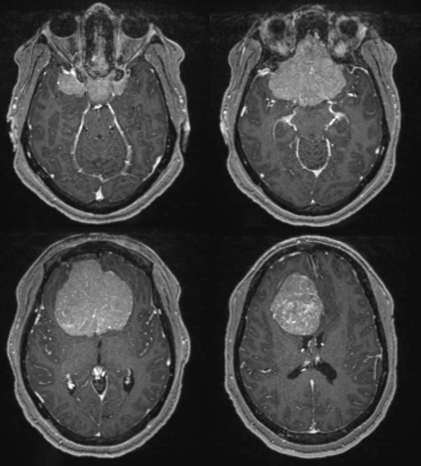
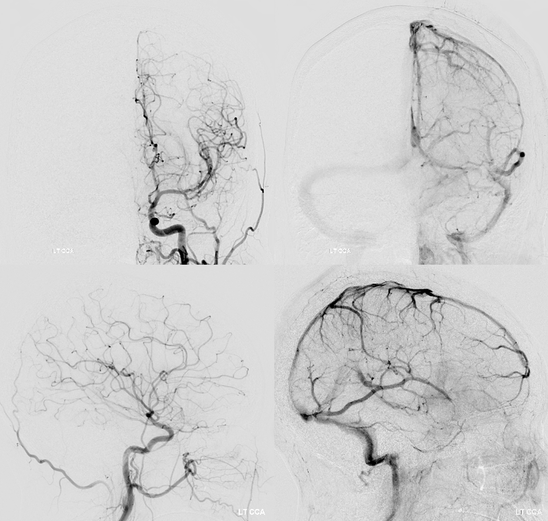
Giant olfactory groove meningioma, preoperative angiogram
Note how far back the tumor extends, enveloping both terminal ICAs and A2s
Angio 2D — not too useful. Usual supply from ethmoidal arteries. not too vascular
Now lets look at the DYNAs
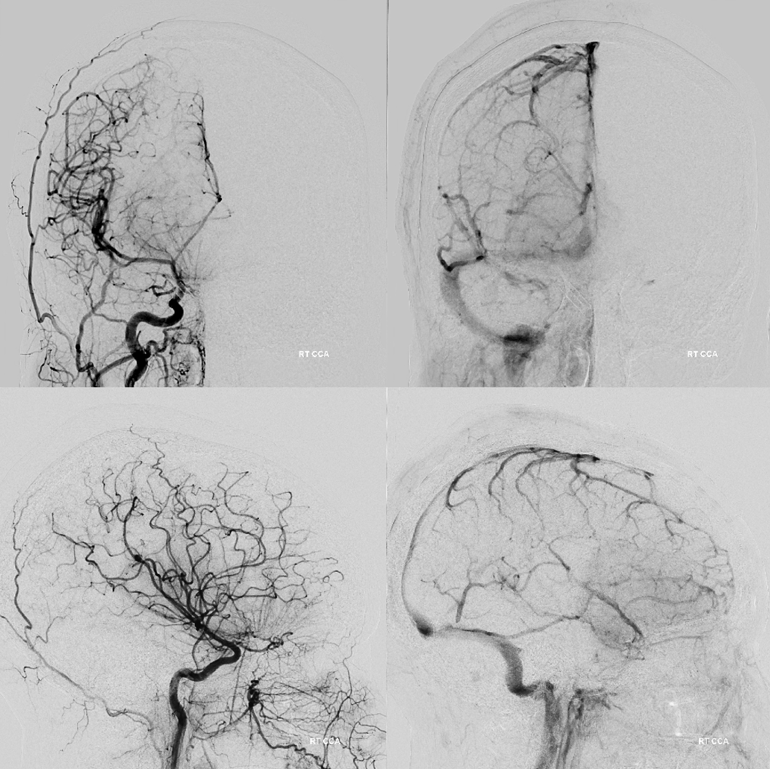
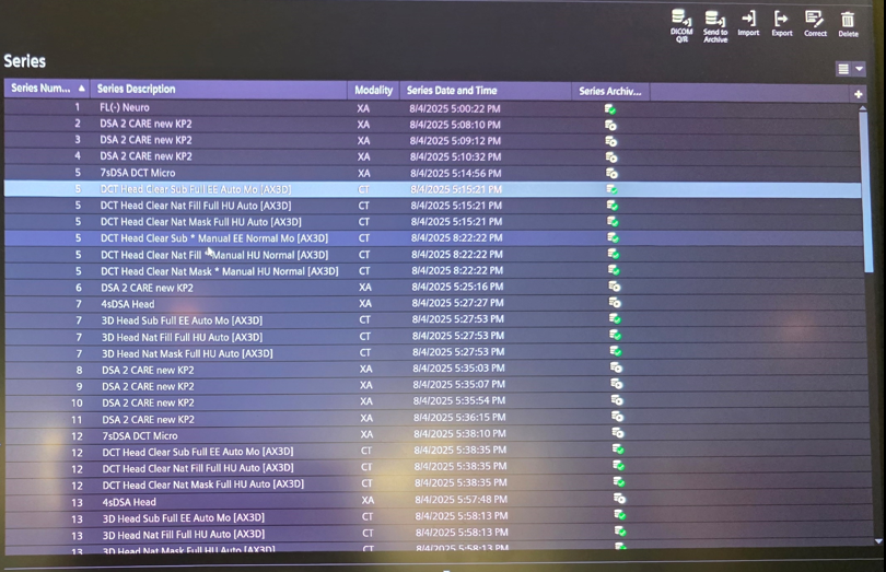
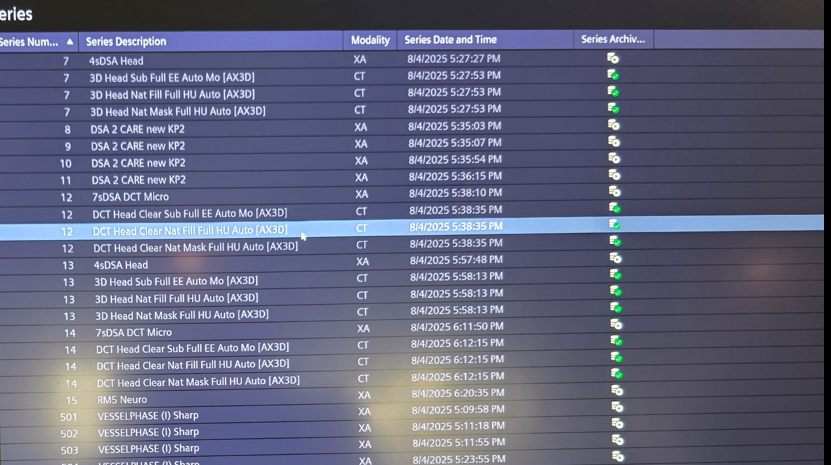
Below is a rare example of all of them being stuck together — one after another. Another lovely error of the error-riddled Icono. It sent them this way to PACs, so we can see them all… Arterial and venous
Now, lets unpack it. First we do the arterial spin of the right CCA
Siemens ICONO 7 second dual volume (DSA DCT) 22 cm FOV non binning “micro”. Injection — 4 cc/sec for 40 ccs, 3 sec delay, 100% contrast
This is the MIP of this acquisition. Wealth of data here. Note enlarged superior hypophyseal for example. Main supply from posterior ethmoidal, with some from ILT and deep recurrent meningeal
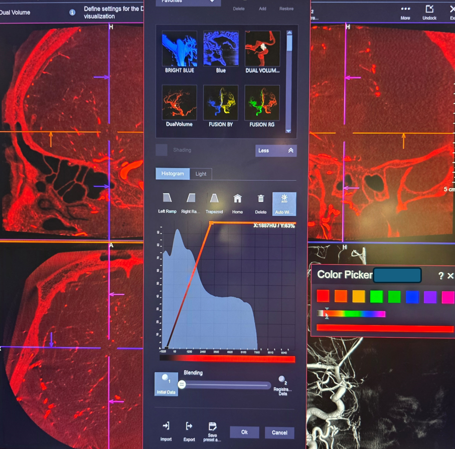
This is the volume rendered reconstruction
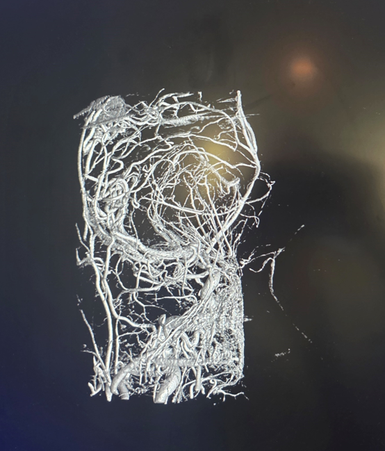
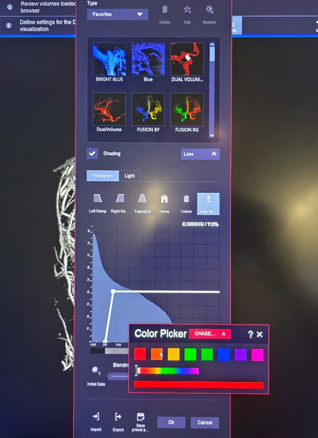
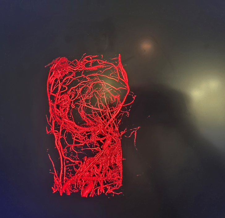
We change the color
Below the rotational VR dataset
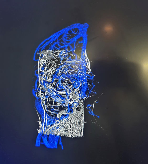
VENOUS VOLUME RENDERING
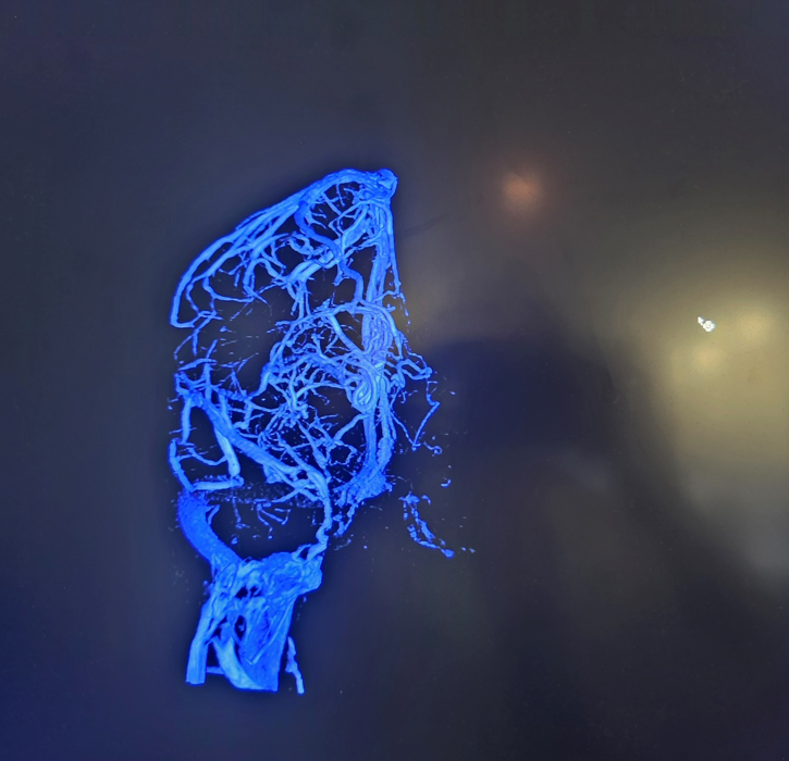
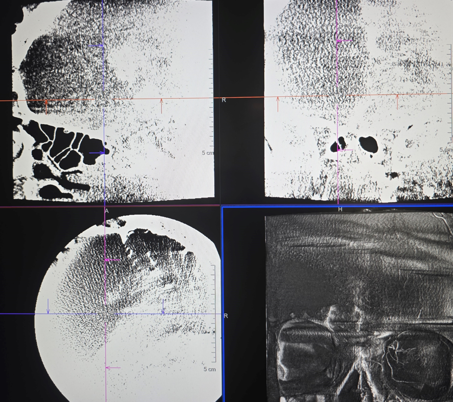
Now, lets say you wanted to get a venous phase dataset, without arterial admixture, like the one below:
How to do this? Not so hard. Because the venous phase is limited, we are limited to 4 second rotational angiogram in the ICONO and 5 second in the Q and Z. So we will choose 4 sec DSA DCT as the protocol.
Now what is needed is the right injection rate and delay
The key is to have the right delay. How to calculate delay? You need to know the amount of time between the END of the arterial injection and appearance of veins. The best way to do this is to set your framerate to 2 frames/second. Not one of those variable framerates of 3-2-1 depending on time etc. We prefer constant rates. So, lets say you have a 2 frame/sec rate. Lets say you inject contrast into the ICA, starting with frame 7 and ending with frame 12 (thus you have injected for 2.5 seconds). So, if the last frame where you see arteries is 12, and you see good venous opacification starting with frame 20, then the delay between end of arteries and good veins is 8 frames or 4 seconds. OK? Good.
Now, to see veins well you need to inject enough contrast into the artery. Typically, for an ICA injection, this is around 12-15 ccs of undiluted contrast, injected at a rate of 3 cc/sec. So, lets do this: 3 cc/sec for 15 ccs total takes 5 seconds. After these 5 seconds, we must wait another 4 seconds to make sure contrast is washed out of arteries, as we determined above. Thus, the delay is 5+4 = 9 seconds. Get it? Good. Don’t ask about how veins will appear earlier because after 5 seconds of arterial injection you should see them already etc etc. The point here is to see veins well, which means filling the arteries for longer than usual.
If this is too confusing, the rule of thumb is ICA injection 3 cc/sec for 15 ccs and 9 second delay. For vert its the same 🙂 — as long as you have a big enough vert.
This is the result for the right side
The same thing on the left side
Below is the Volume Rendered reconstruction produced from this dataset
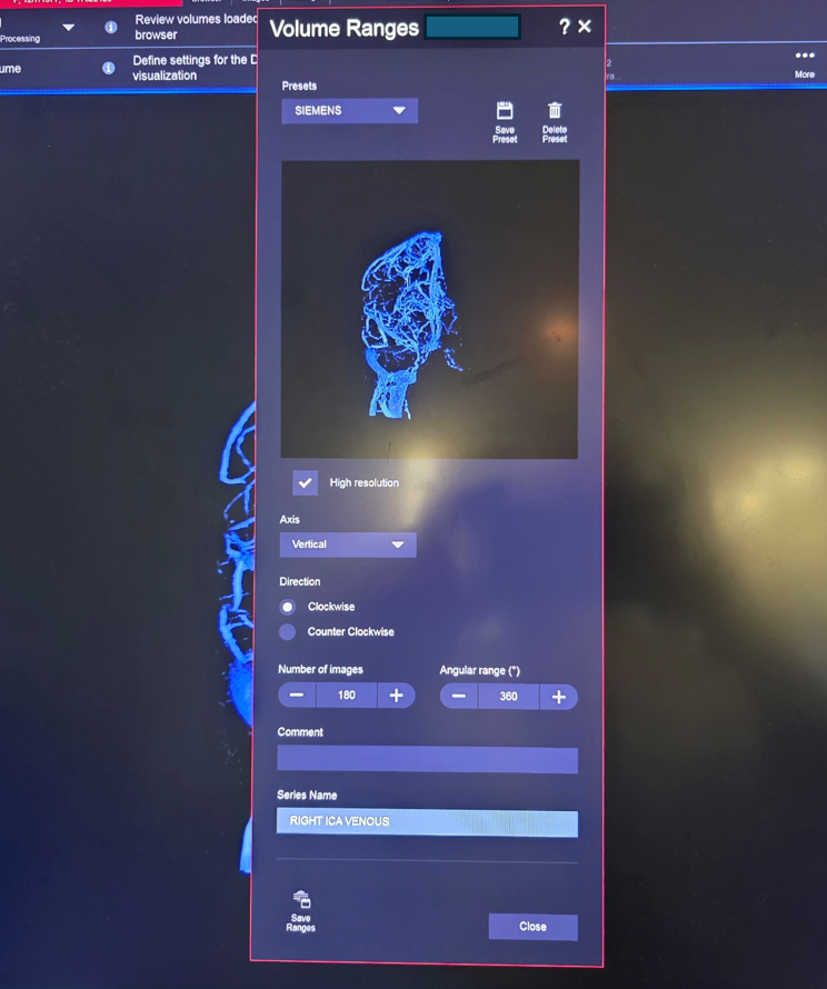
We produce a rotational dataset like this. There are 180 images for allround 360 degree angular range.
This is the result:
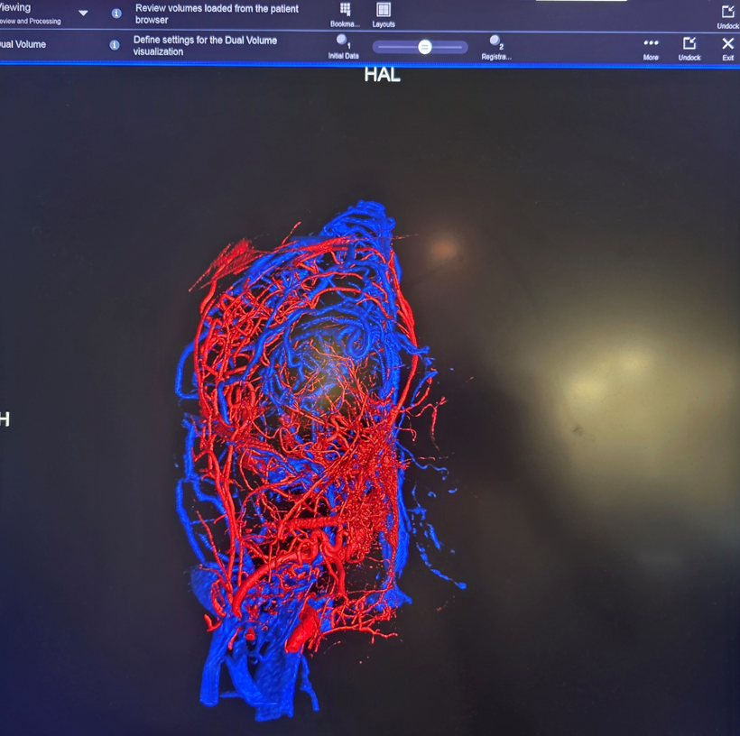
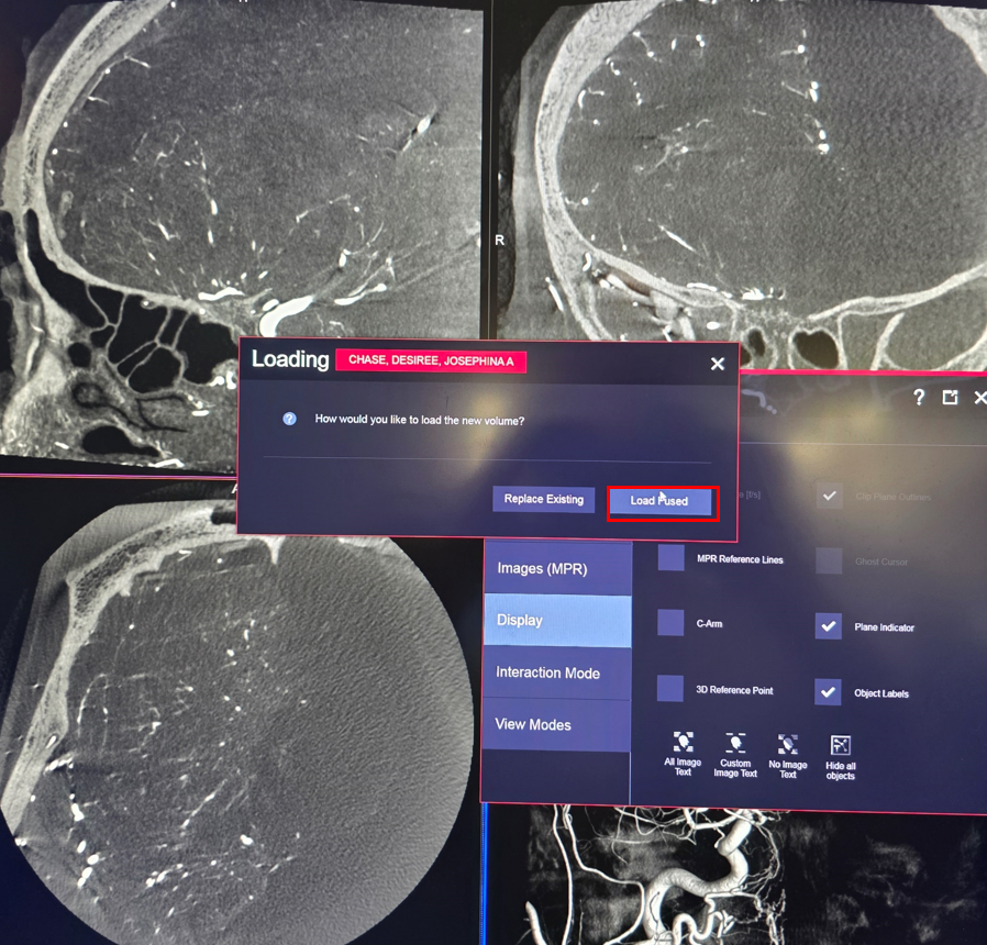
Now, we want to fuse the arterial dataset with the venous one. We keep the venous database and add the arterial one
Choose “Load Fused”
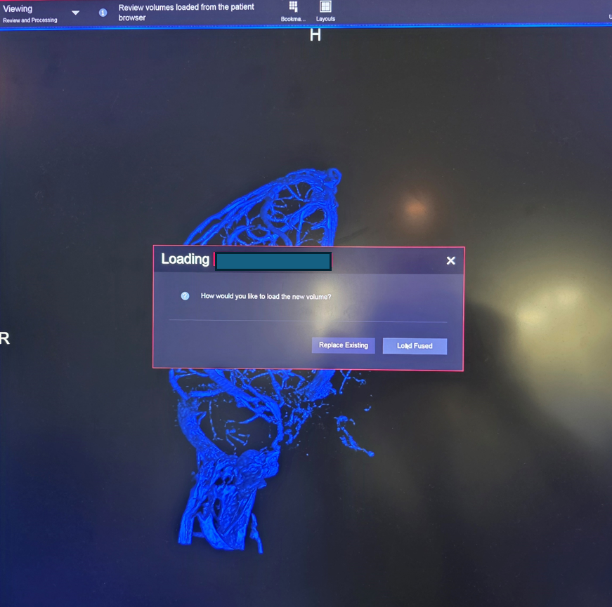
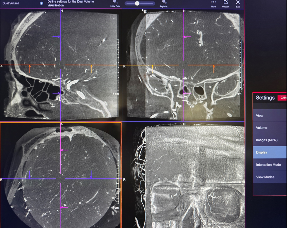
This is what happens. We need again to change color of the arterial dataset
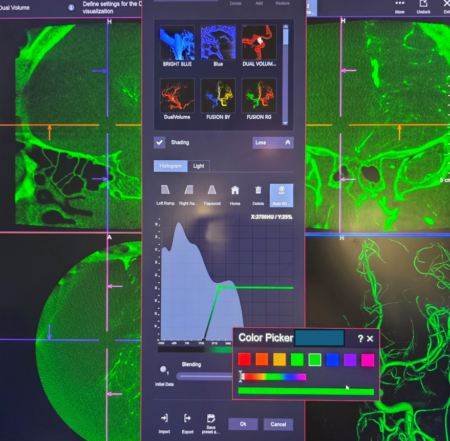
We select the arterial dataset and change color
This is the result
We now create a rotational VR dataset
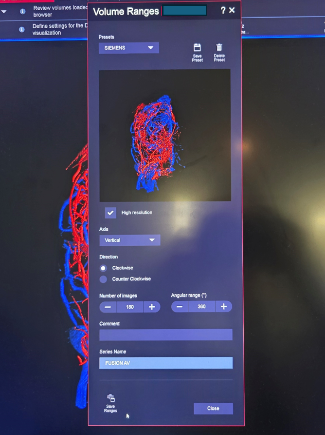
This is the result
This concludes the review of how to fuse arteriovenous images.
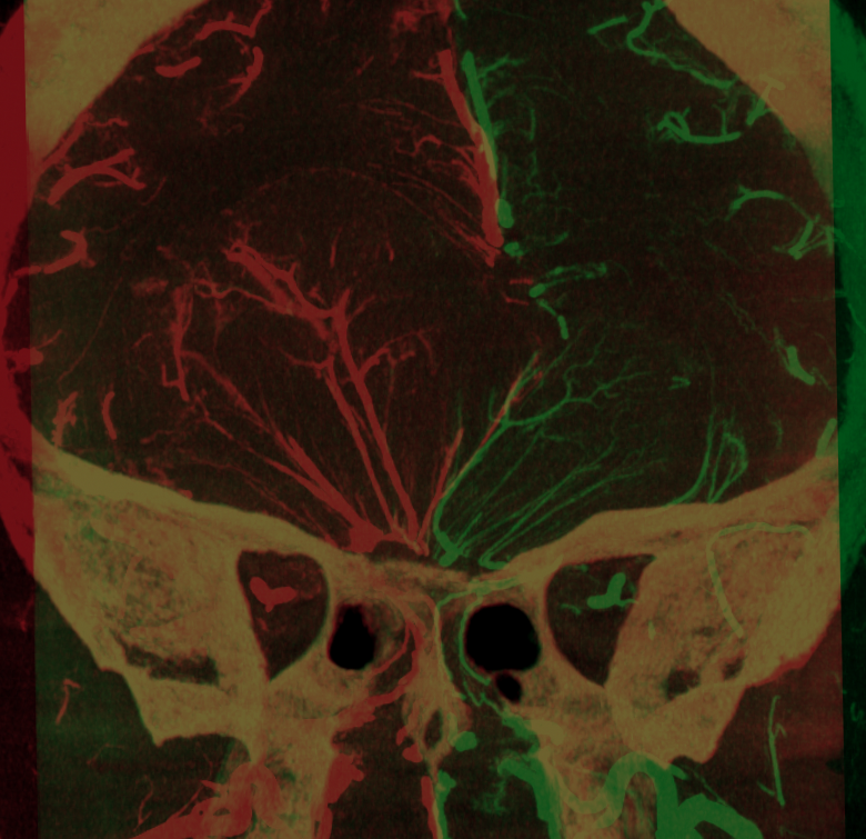
Now, we can fuse the right and left CCA “natural fill” arterial datasets together as well, to understand arterial supply, like this:
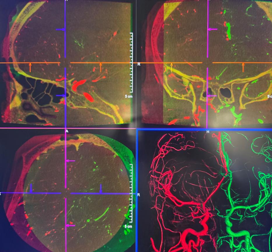
Fusion MIPs
How to do this? Same way
Take one of the “Natural Fill” datasets
Add the left CCA one
Get this result. “Load Fused”
Get this result
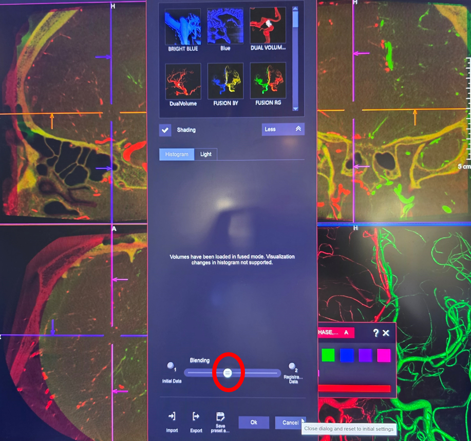
Change windowing
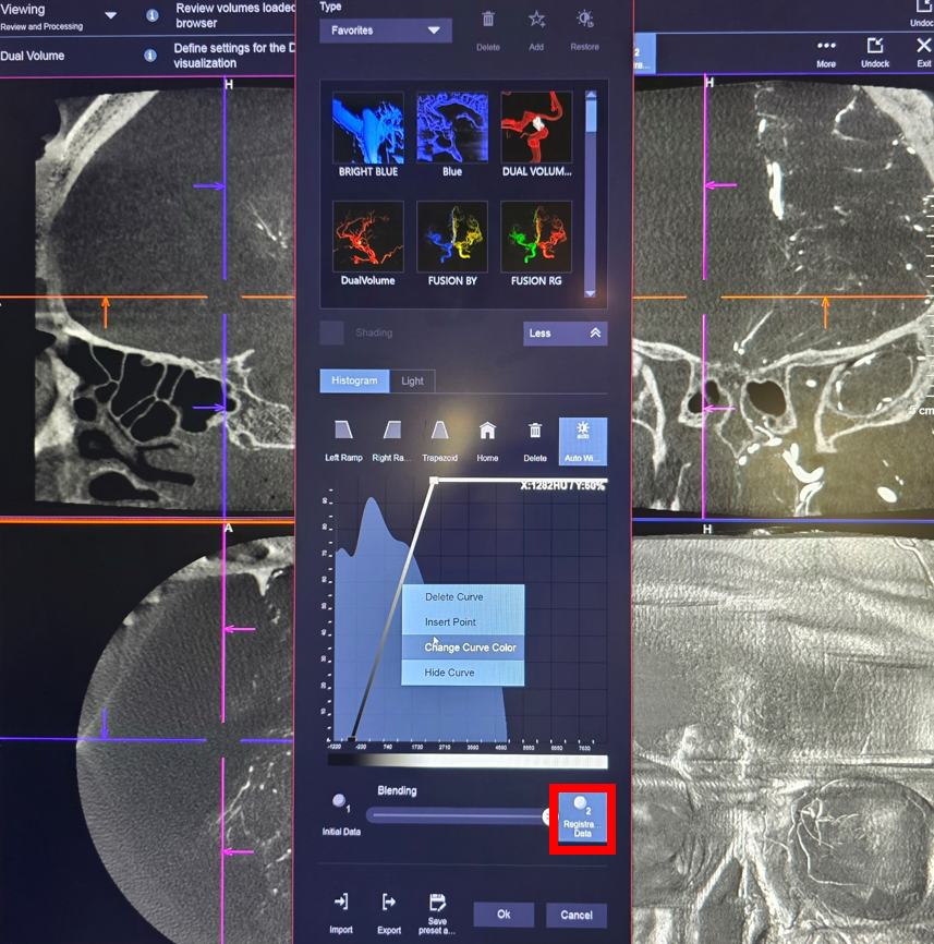
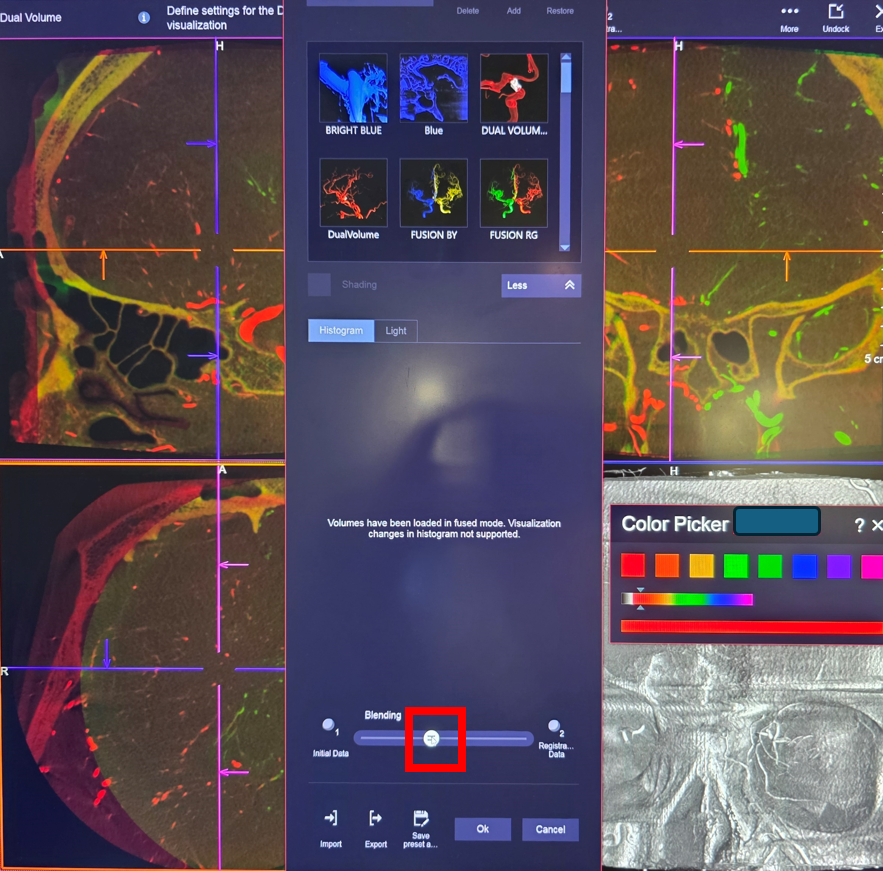
Change color of MIP by selecting either the “Initial Data” or the “Register Data” (red square) to change colors in each dataset separately
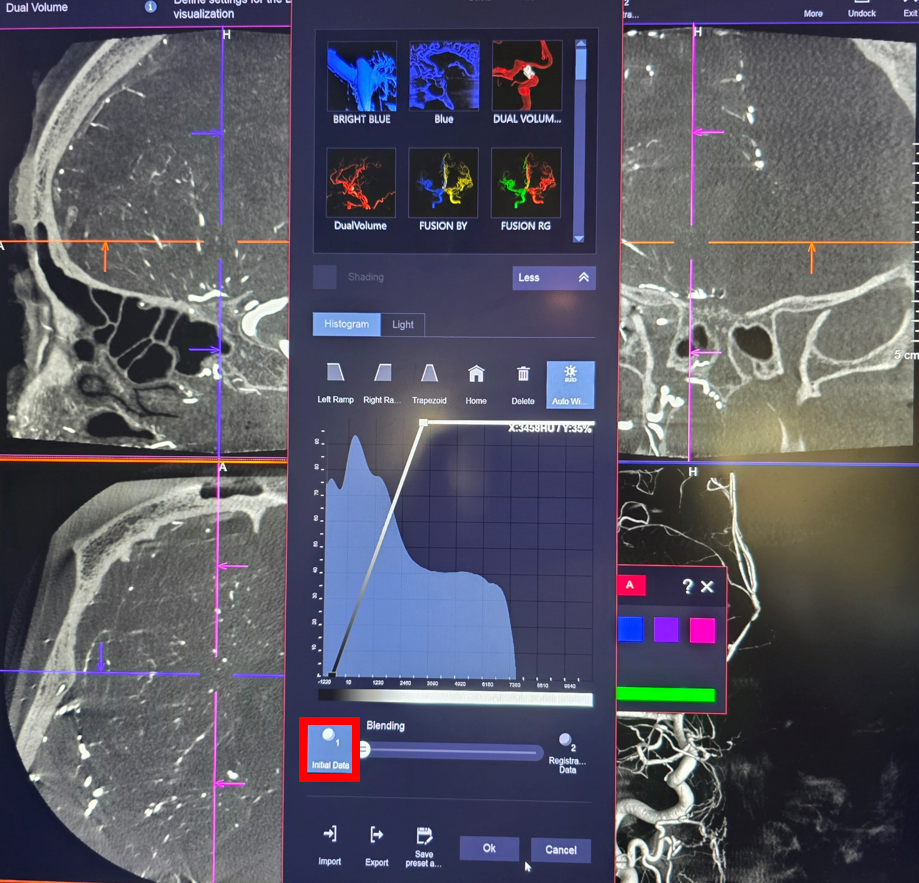
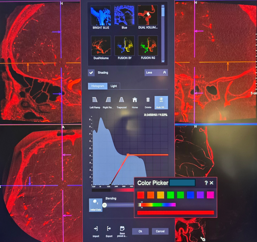
Now go to the right ICA (the initial dataset)
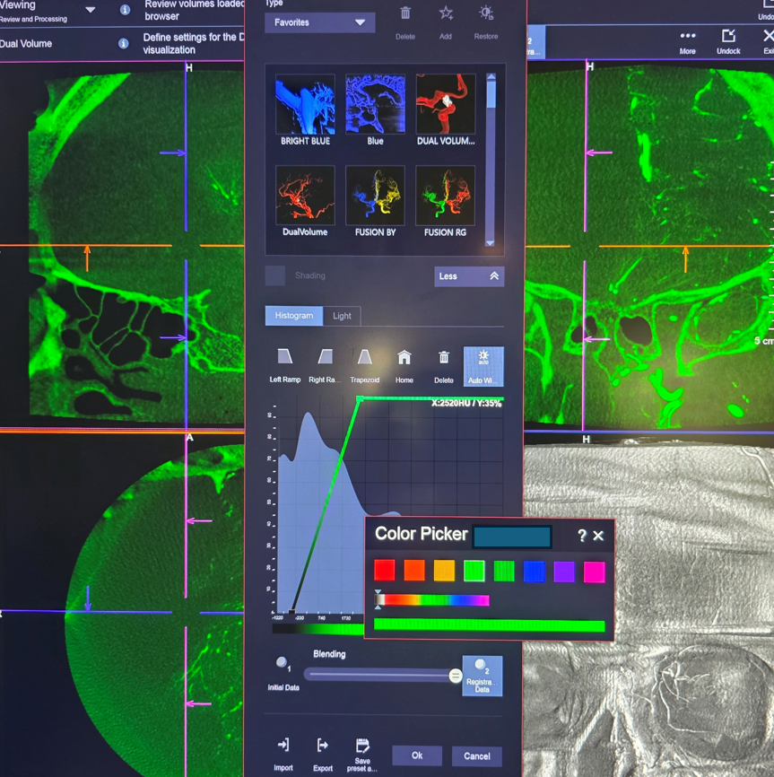
Change that to red
Blend together (red circle)
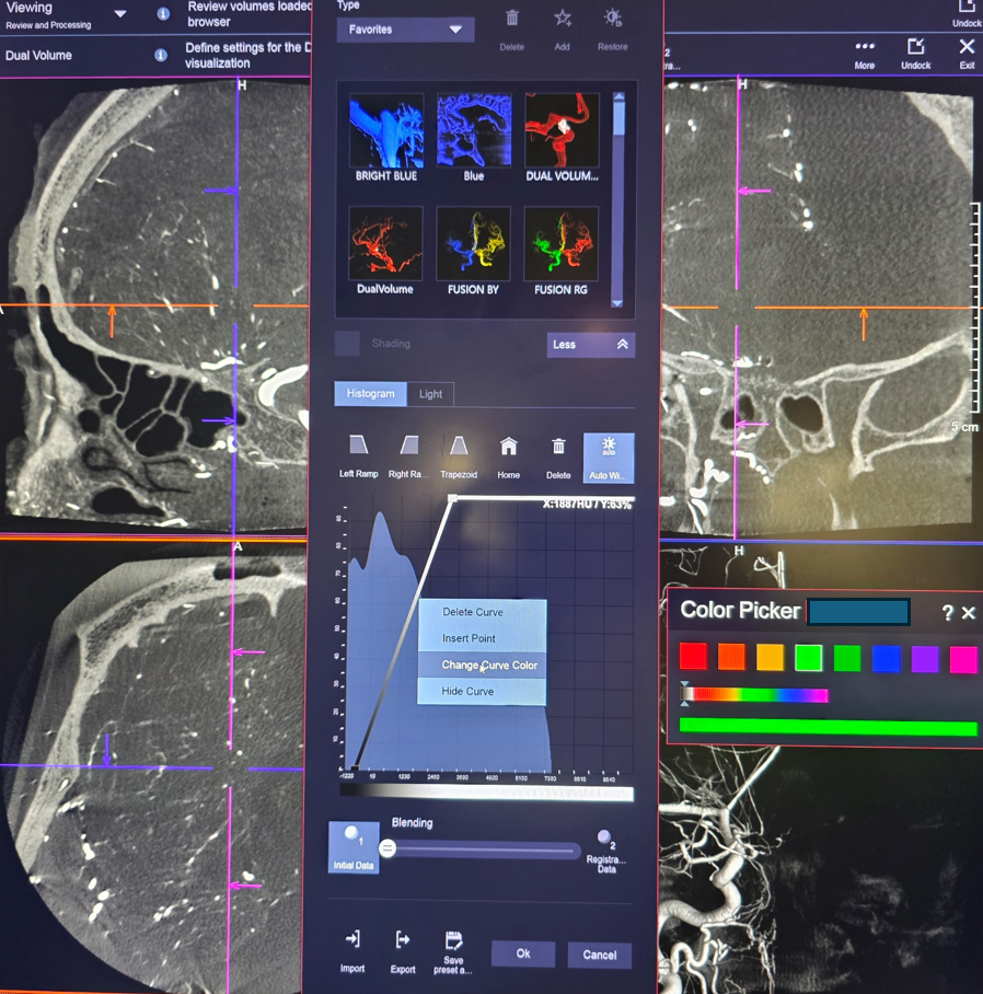
Change colors for the Volume Rendered set by clicking on it and repeating the same thing
Blend VR datasets
only twenty steps later…
Vary Image thickness in MIP dataset to your liking
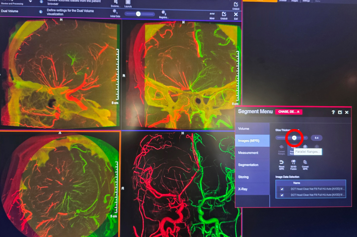
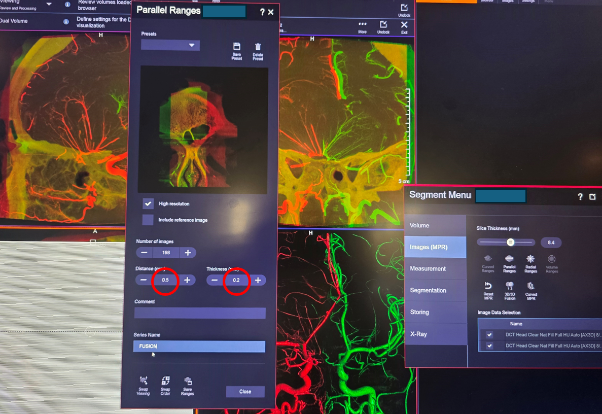
Make Parallel Ranges of MIPs. Vary slice distance and slice thickness to your liking
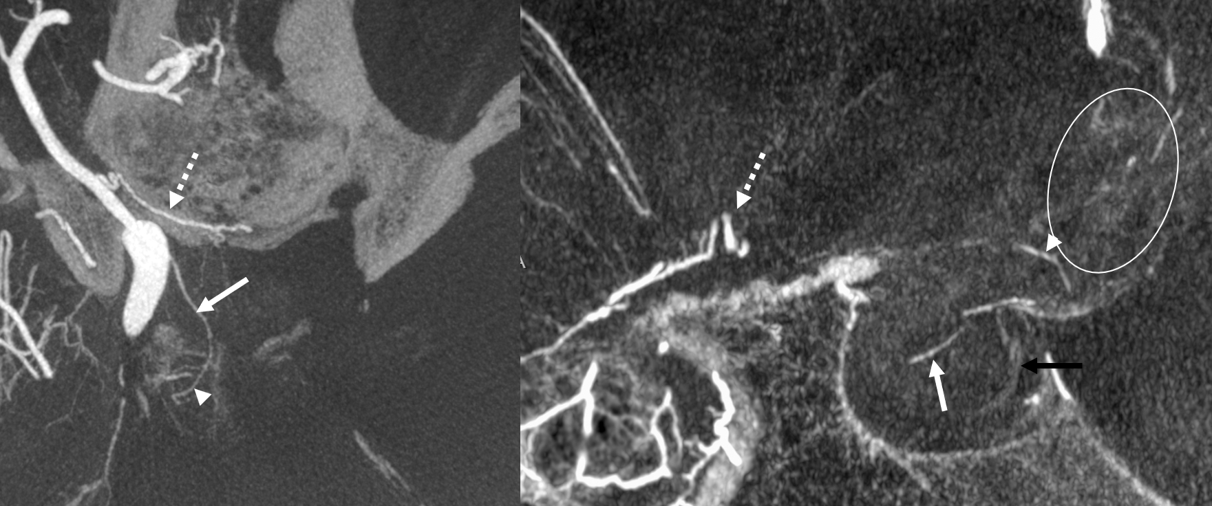
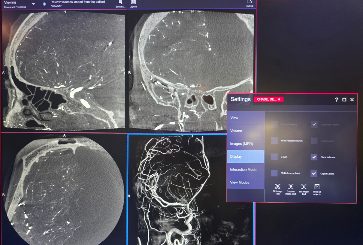
Below are the MIP datasets
Much more is there than colors. For example, the right superior hypophyseal artery is hypertrophied (arrows), with its distal portion (arrowhead) recruited into supplying the tumor (white oval). Further supply to tumor is from deep recurrent meningeal artery (dashed arrows). The pituitary is posteriorly displaced within the sella and above it (black arrow)