
This section is created by Rahul Kumar, MD; Patna, Bihar, India. CEO at G S Neuroscience Clinic and Research Centre Private Limited
What is Catheter Cone Beam CT Angiography (CBCTA) ?
This term is used colloquially in the Angio suite but let us take a step back and try to understand the origin of this term. For this, we must first understand the working principle of a conventional CT scanner and then try to apply the same knowledge to the Flat Panel Detector (FPD), and in the process try to understand the differences.
Conventional CT Scan Physics and technique
Depending on the generation of CT scanner being used, the physics and the hardware are configured differently. In the oldest clinically available models, the X-Ray source used to be a point source and it used to shoot a single beam through the object that used to be picked up by a single small detector, and then the whole construct used to move around the object and keep on repeating the process (Fig 1)
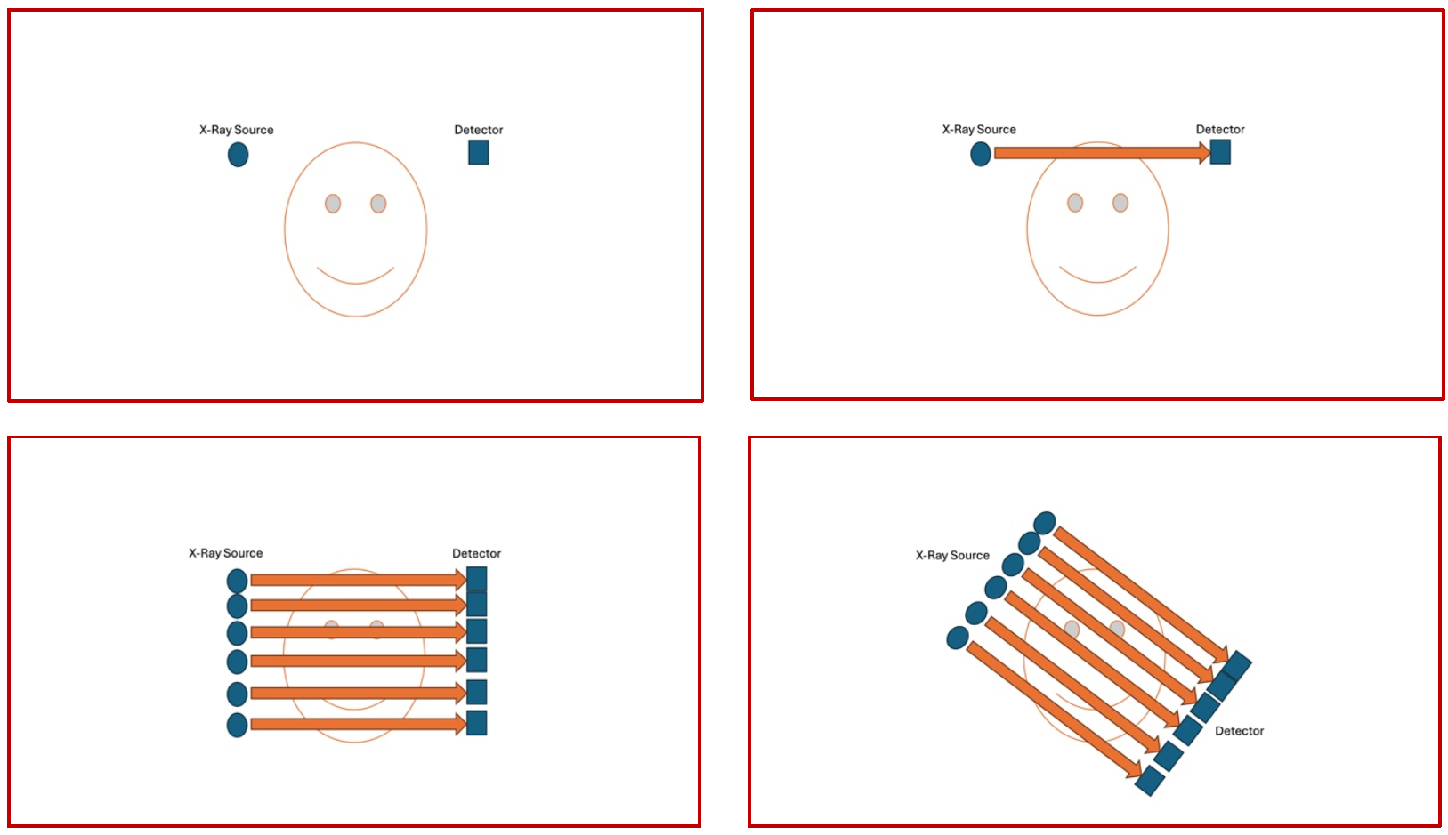
(Fig 1 – Conventional 1st generation CT Scanner – the X-Ray source is seen on the left and the detector is seen on the right of the panel. The source emits a single beam that is captured by the detector, then the process continues to acquire parallel slices. Once the entire object has been X-rayed, then the entire construct moves by an angle of the arc and the whole process is repeated till the entire circumference is acquired.)
As it will be very obvious from the images shown here in Fig 1 (a poor attempt to demonstrate something quite so complex !!), the entire workflow of the first-generation scanner is very slow and cumbersome. This was the only thing available in the late 70’s and early 80’s.
Fast forward a couple of decades and now we are in the era of the 4th generation scanners that are widely used for clinical purposes. (Fifth generation photon counting, electron beam scanners are also available but that remains another discussion). The main differences that are seen in the fourth generation scanners is the presence of a circumferential detector around the patient in the gantry ( which remains stationary ) and a point X-Ray source that spins around the patient in a continuous fashion acquiring the images as it rotates (Fig 2).
(Fig 2 – 4th generation CT Scanner – the X-Ray source is seen on the left and the detector is seen circumferentially around the object being scanned. The source emits a single beam that is captured by the circumferential detector and the source keeps on moving continuously around the object being scanned )
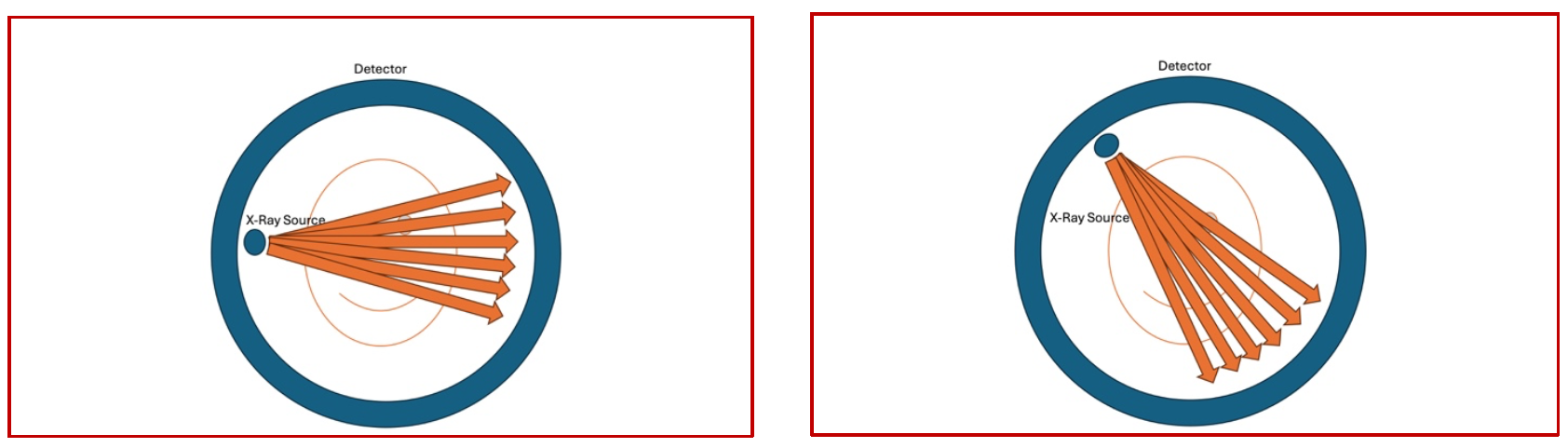
In essence, despite the major differences in the construct and workflow of different scanners, one principle remains fairly constant in conventional CT scanners. Since a point source is used as the X-Ray generator and a single detector moving in an arc(1st gen) or a point source as the X-Ray source with a circumferential detector (4th gen), the distance travelled by the x-ray beam from source to destination, through the object, remains constant. Due to this, the shape of the beam as it transcribes its orbit is almost like a fan in shape, and therefore the conventional CT scan is also called as the “Fan Beam CT” (Fig 3)
(Fig 3 – as the image is generated in a conventional scanner, each of the X-Ray beams labelled a, b and c emanate from the generator, pass through the object and reach the curved detector. Since the origin is a point and the destination is curved, the length travelled by all the three representative beams remains the same. Therefore, the sector being scanned has a fanlike shape, with the narrowest point at the origin of the beam and the terminal part remaining curved )
So, What is Cone Beam CTA ?
Now that we have understood the generation of conventional spiral CT, it is the right time to apply these principles in the angio suite. As we are all aware, neither is the detector in the angio suite a doughnut shaped circumferential detector, not is the detector curved like we see in conventional CT. The X-Ray generator remains almost identical, just miniaturized in size, to oversimplify things. The main differentiating point is in the Flat Panel Detector. As the name suggests, it is flat instead of being curved and this makes things different, and interesting.
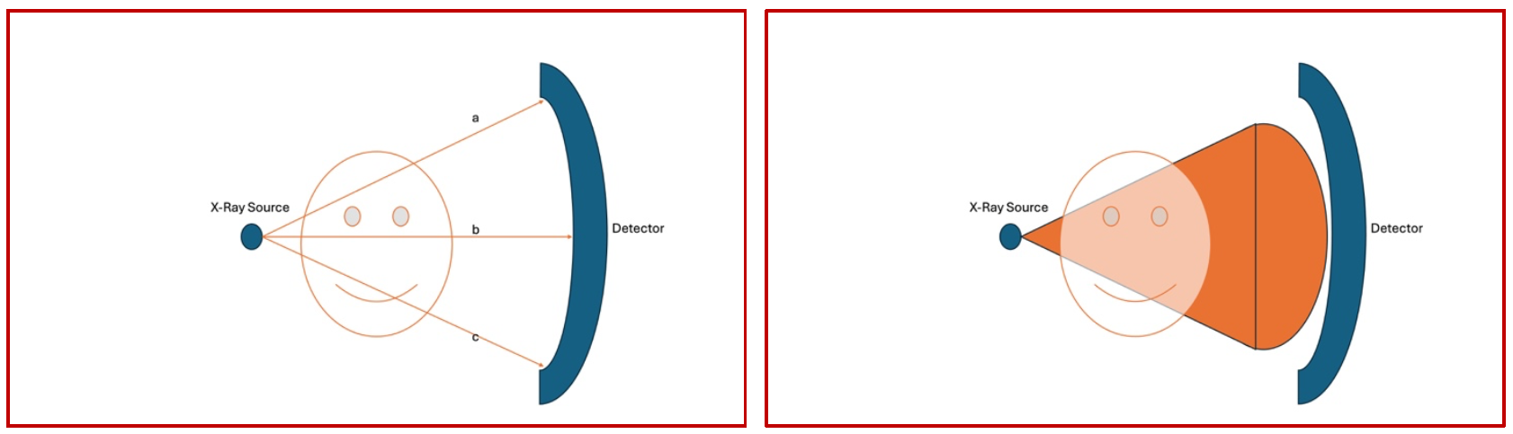
The basic principles remain as in spiral CT. There is a source, there is an object and there is a detector. Also this is where the similarities end. The imaging principles have been summarized in the following image (Fig 4)
The sector that is transcribed by the scanner in a flat panel detector, unlike in a curved detector, takes the shape of a cone instead of a fan, and therefore any CT acquisition using a flat panel detector, is essentially a Cone Beam CT Exploration.
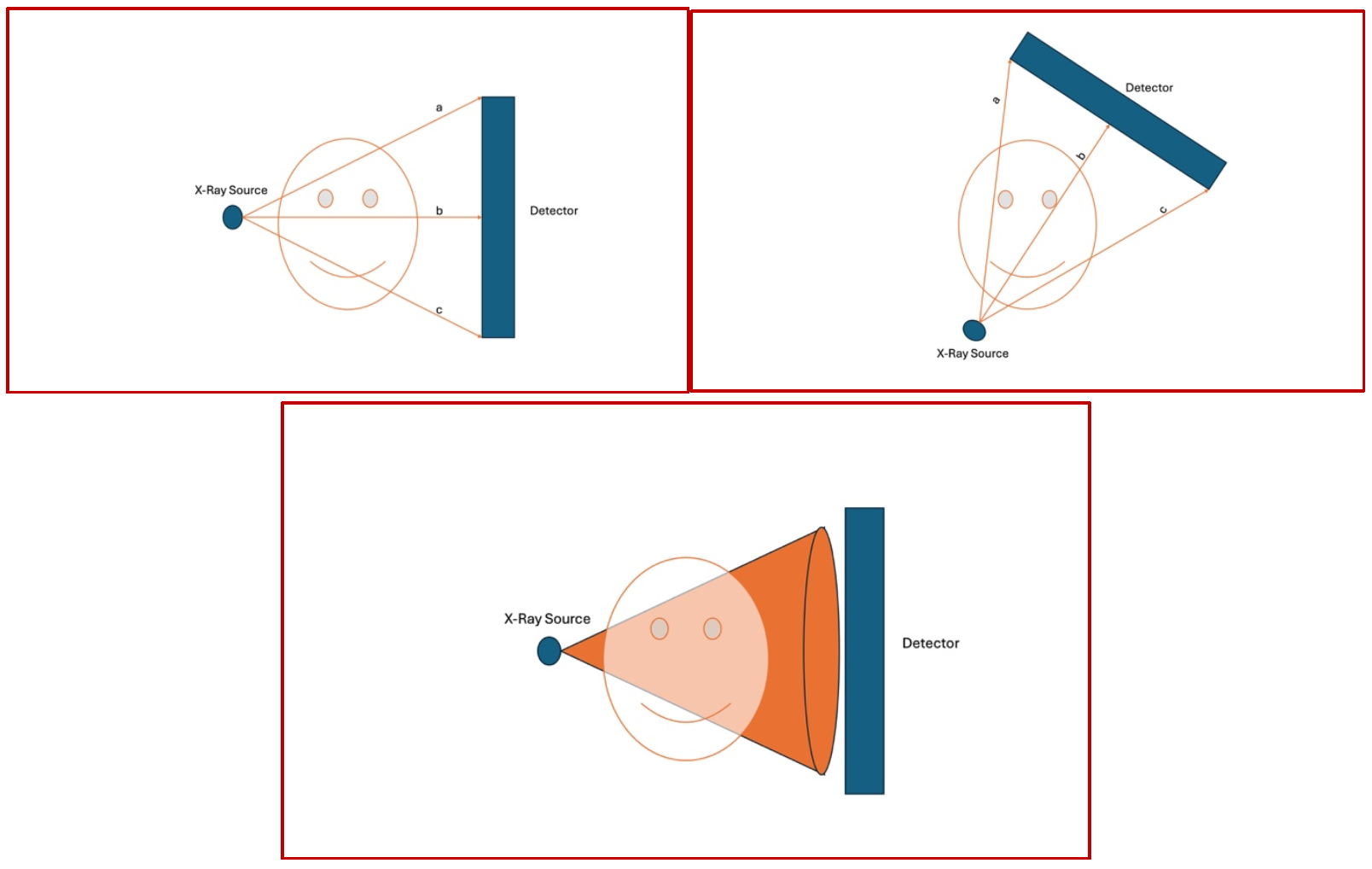
(Fig 4 – as the image is generated in a flat panel scanner, each of the X-Ray beams labelled a, b and c emanate from the generator, pass through the object and reach the flat panel detector. Since the origin is a point and the destination is flat, the length travelled the two peripheral beams a and c is considerably longer than the beam in the center of the field, b. Therefore, in this flat panel situation, the sector being scanned has a conical shape, with the narrowest point at the origin of the beam and the terminal part of the scanned sector remaining flat, like the base of a cone)
Conversion of X-Rays into a 2D and subsequently in a 3D image set – how does it happen ?
As we have discussed in the previous sections, in essence, all that a CT Scanner does is shoot an X-Ray beam through an object, and that beam gets to travel through the object and finally get picked up by a detector. On its way to the detector, part of the beam gets reflected, part gets absorbed/modulated in terms of its frequency and part gets to go through and through. It is this modulation that is interpreted by the detector as varying densities (Fig 5).
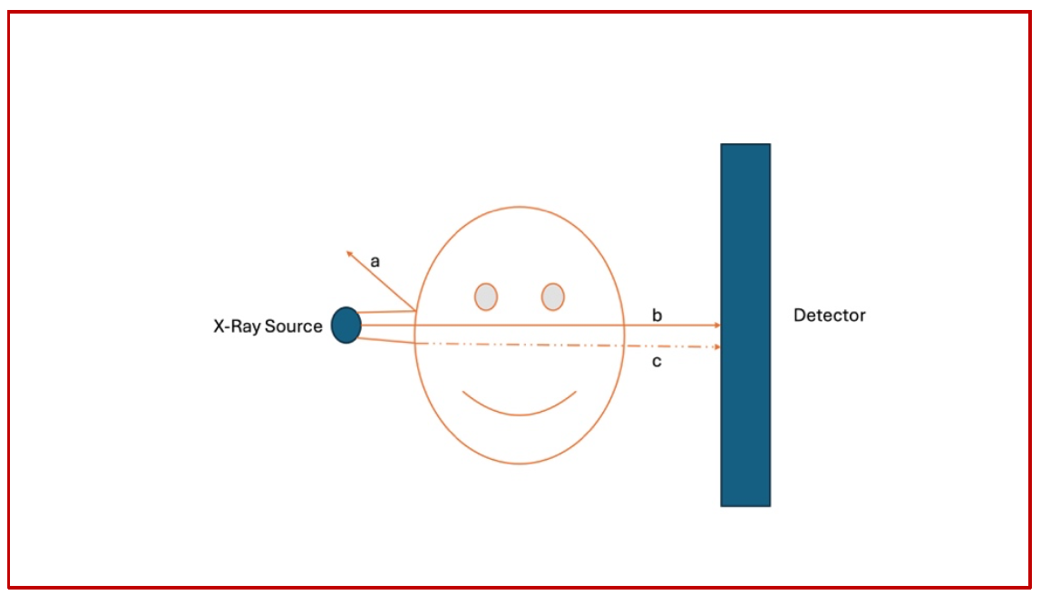
(Fig 5 – Three representative X-Ray beams named a, b and c are shown here. Beam a does not penetrate the object at all and gets reflected completely back and does not reach the detector. This is the reason for the so called “scatter radiation” in the angio suite. Beam b passes through in its entirety and reaches the detector almost unchanged. Finally, beam c, upon entering the object, gets partially absorbed by the object and a portion of it gets to reach the detector.)
Once this concept is clear, we can begin to build on this and understand how this gets converted into a grayscale representation at the end of the pipeline. The key point here is that at the end of the acquisition, there will be a set of numbers generated by the detector all around the object, and these numbers will essentially be the intensity and frequency of the x-rays that have made it to the detector (Fig 6)
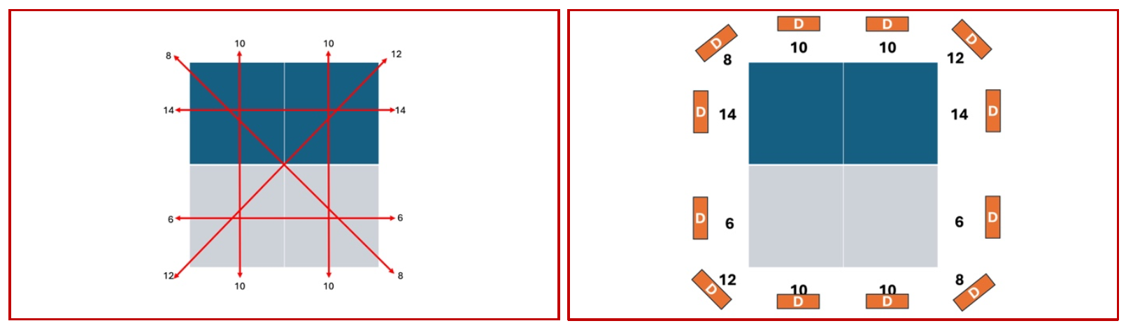
(Fig 6 – The left-hand panel shows the multiple hypothetical locations from where the images have been acquired. The panel on the right-hand side shows the arbitrary numbers picked up by the detectors (D) all around the object of interest.)
Once these numbers, that actually represent the X-Ray attenuation values circumferentially around the object of interest have been acquired, it becomes a matter of simple mathematics to reverse-calculate the values of the boxes that lie within this area.
The more the number of directions at which the data has been acquired, the more is the number of hypothetical squares that can be generated within the area of interest; the more this number, the better is the image. Once the data has been calculated for each square within the area of interest, it is given a value on a grayscale gradient, and the computer converts this into an image of multiple small squares, called pixels, of varying densities. The composite from this is the final CT scan image that we know of and use daily in our clinical work (Fig 7). Each pixel, depending on the sophistication of hardware can be of varying sizes, and this ability to image very small pixels improves with improvements in hardware and software developments. Each pixel represents an area in the anatomy that is being studied, and this part of the body that is represented by a single pixel is called a voxel.
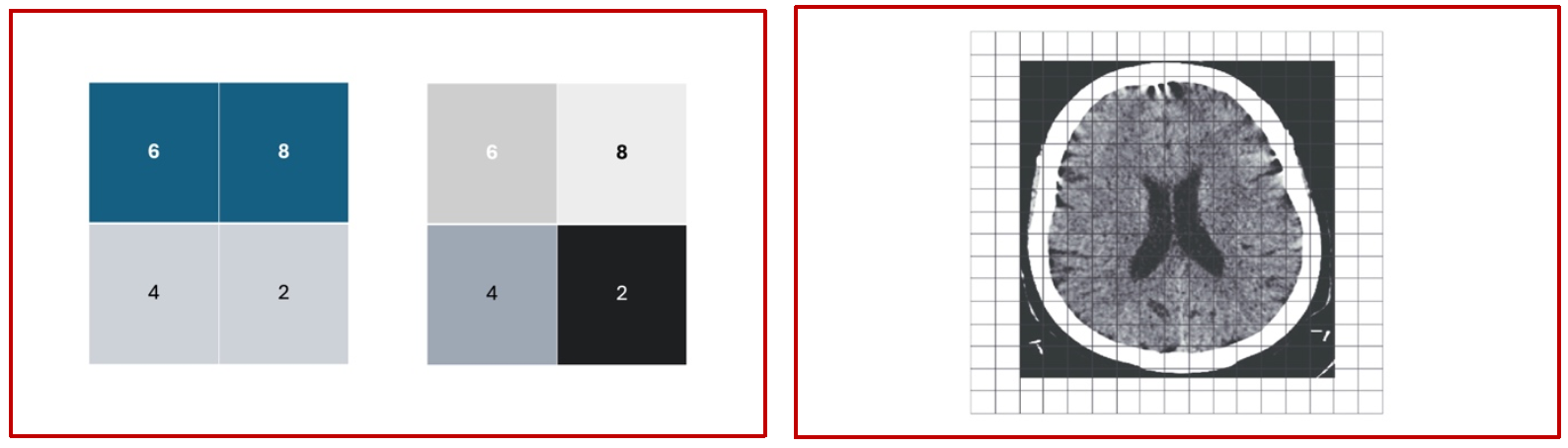
(Fig 7 – The panel on the left hand side shows the reverse calculation of the attenuation values of the individual pixels and their conversion into a grayscale format, and the panel on the right hand side shows the conceptual application of this principle in the final generation of a collection of pixels of varying shades from white to black, finally giving rise to a cross sectional conglomerate of pixels representing an anatomical structure)
Post processing – the concept of “binning”
Now that we have understood how images are generated, and how voxels are converted into pixels, we also need to understand that the images that are presented to us for clinical use are not the same ones that have been acquired using all the principles that we elucidated earlier, in the sense that a lot of post processing goes in between the raw dataset and the finished image on the console. One of the techniques that is used almost universally is “binning”. Let us understand what this is.
The raw dataset out of the scanner at the point of acquisition, especially in the current generation of machines contains too much data for a smooth image. The initial pictures are typically very noisy as the pixel sizes are very small. To circumvent this noise in the final image, developers devised a technique by which the adjacent pixels are merged and the densities are averaged, giving origin to larger pixels and more uniform densities, thereby reducing the noise in the image. While in most cases this does not impact the clinical interpretation and diagnostic use of the data, in situations where we need very high spatial resolution and noise is not much of a concern, unbinned data sets are preferred over binned data sets. The following illustration summarizes the concept of binning and its application to imaging protocols (Fig 8).
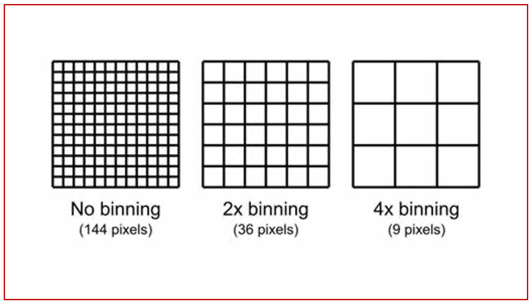
(Fig 8 – raw data acquisition at 12×12 pixels, an arbitrary figure produces a raw matrix of 144 pixels. If this is post processed at 2X, you get a 6×6 pixel format with a matrix of 36 pixels. If the same is post processed at 4X, you get a matrix of 9 pixels).
Flat Panel CBCTA exploration – specifics – the concept of “Isocenter”
The isocenter of a biplane catheterization lab is the theoretical point in space where the central X-ray beams of both the frontal (antero-posterior) and lateral imaging systems intersect. This is marked as a small red dot on both the frontal and lateral planes. Since this is a point in space where the maximum number of beams intersect during rotation of the C-arms, it automatically implies that the maximum amount of data about a given voxel will be generated when this voxel is positioned at the isocenter, both in the anteroposterior and the lateral projections. The following sets of diagrams show the concept of the isocenter as well as the correct way to position the object/area of interest in the correct positions in both AP and lateral projections (Figures 9, 10 and 11). All these concepts will be illustrated in the subsequent sections with real world examples.
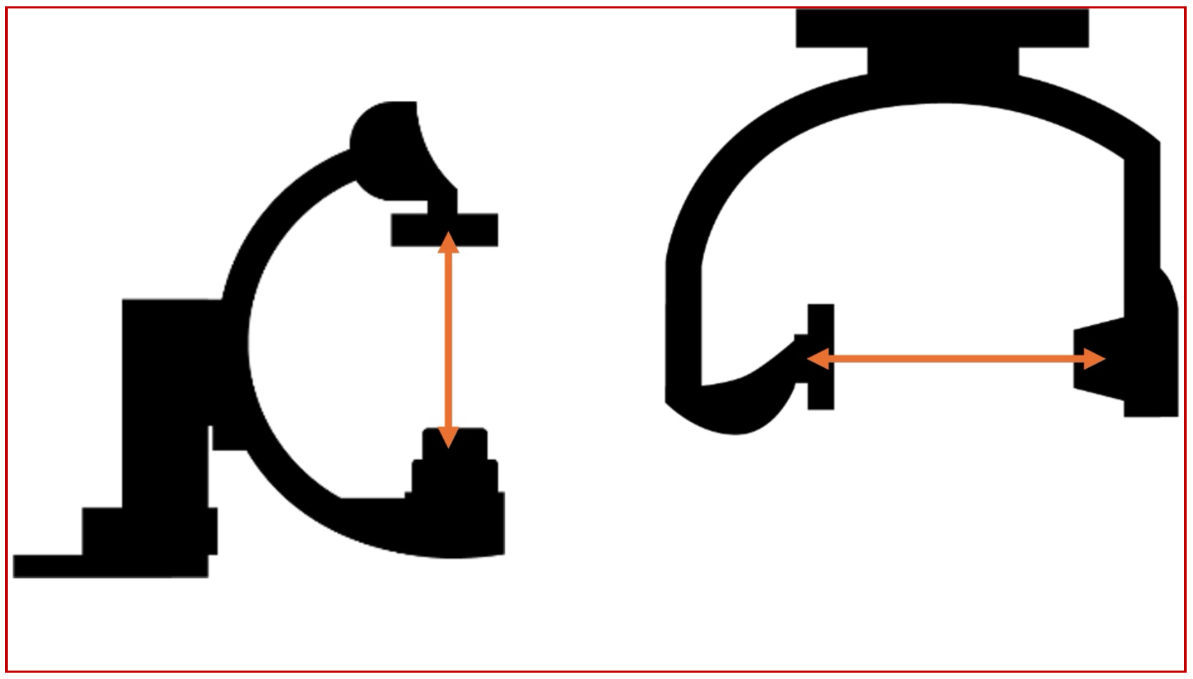
(Fig 9 – the relative positions of the isocenters in the AP and lateral planes, always marked by a red dot on the gantry)
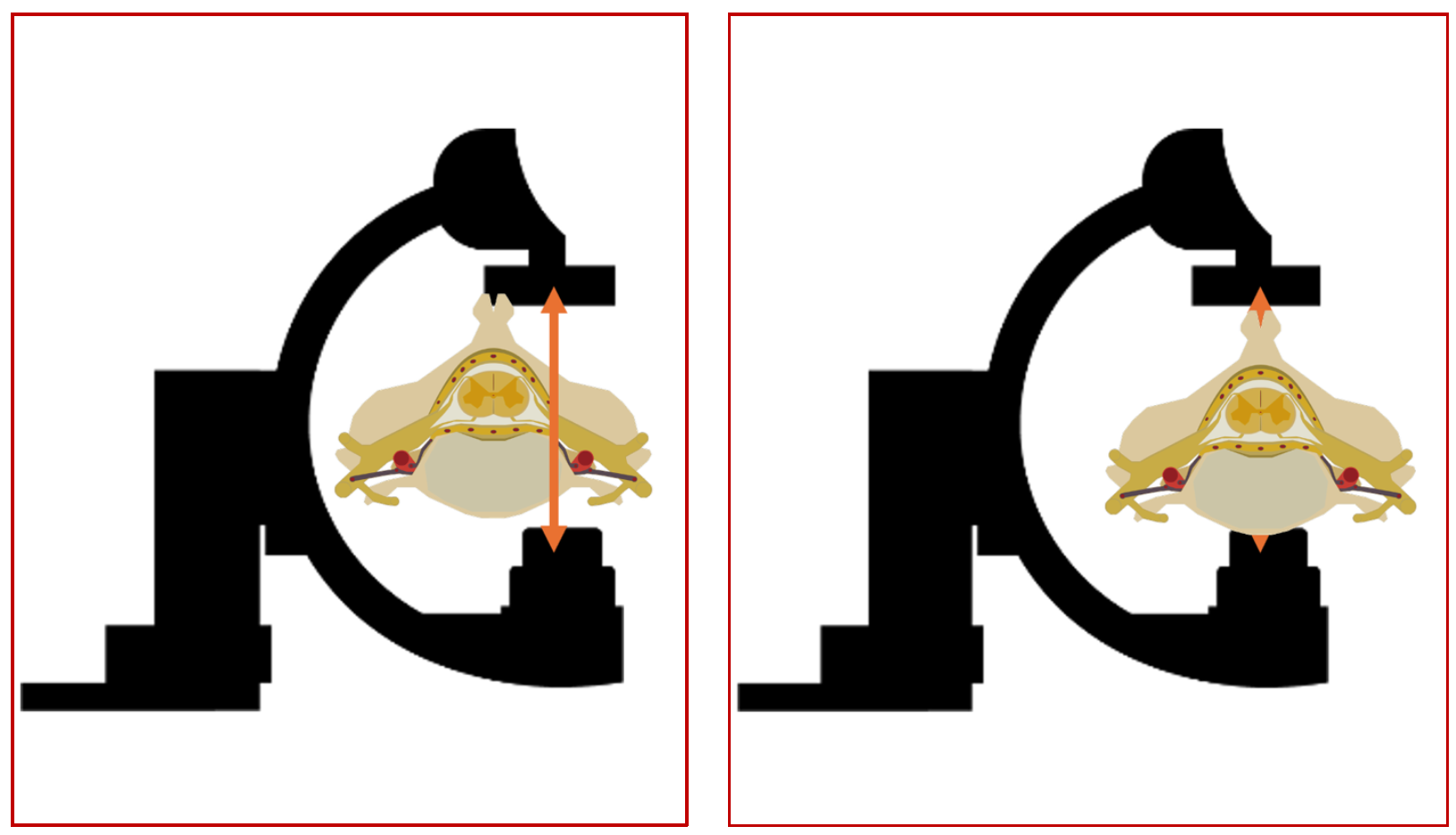
(Fig 10 – Imaging of a small structure like the spinal cord vasculature. The left hand panel showing the oD isocenter location of the area of interest, and the panel on the right hand side showing the correct positioning in the isocenter, thus optimizing the imaging of the spinal vasculature)
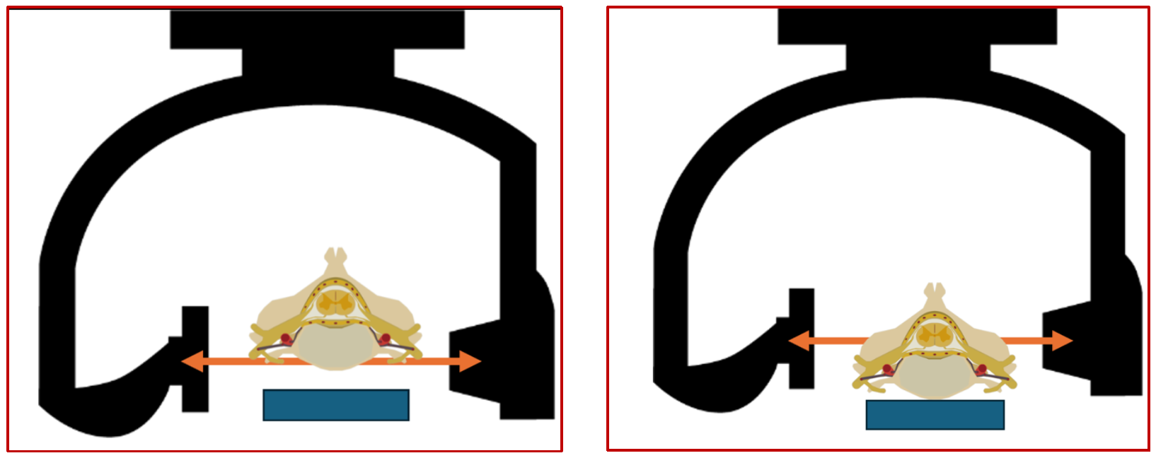
(Fig 11 – Imaging of a small structure like the spinal cord vasculature. The left-hand panel showing the oD isocenter location of the area of interest, in the lateral plane. The patients back is not positioned in a way that keeps the spinal canal in the isocenter. the panel on the right-hand side showing the correct positioning in the isocenter, thus optimizing the imaging of the spinal vasculature).
Clinical example illustrating the concept of isocenter
An elderly male patient presented with progressive paraparesis and double incontinence of subacute onset. MRI of the Dorso-lumbar spine showed the typical features of a dural fistula. A spinal DSA was performed which showed the Adamkiewicz originating from the Left T11 and a radiculo-meningeal branch going to the fistula from the same level. No other pedicles were found to be involved. Patient has severe reservations about surgery, and therefore endovascular approach was considered apter a due explanation of the pros and cons. In view of the complex anatomy and the Adamkiewicz from the same pedicle, a CBCT exploration was done to examining the anatomy further for embolization.

The study was performed under general anesthesia and apnea. Despite these fantastic conditions, my fellow who was performing the study was unable to get satisfactory images as seen on the right-hand side panel. The ASA was seen as was the dural branch but there was no clarity. On closed examination of the source images as shown on the left-hand side panel, it was obvious where the problem was. As it can be seen with the imaginary isocenter lines superimposed, the area of interest was mush much below the point of intersection and thus the image quality suffered.
The study was repeated with the attention being paid to these issues and the images obtained were radically different, with much better delineation of the anatomy, despite using the same physical conditions, image is shown below.
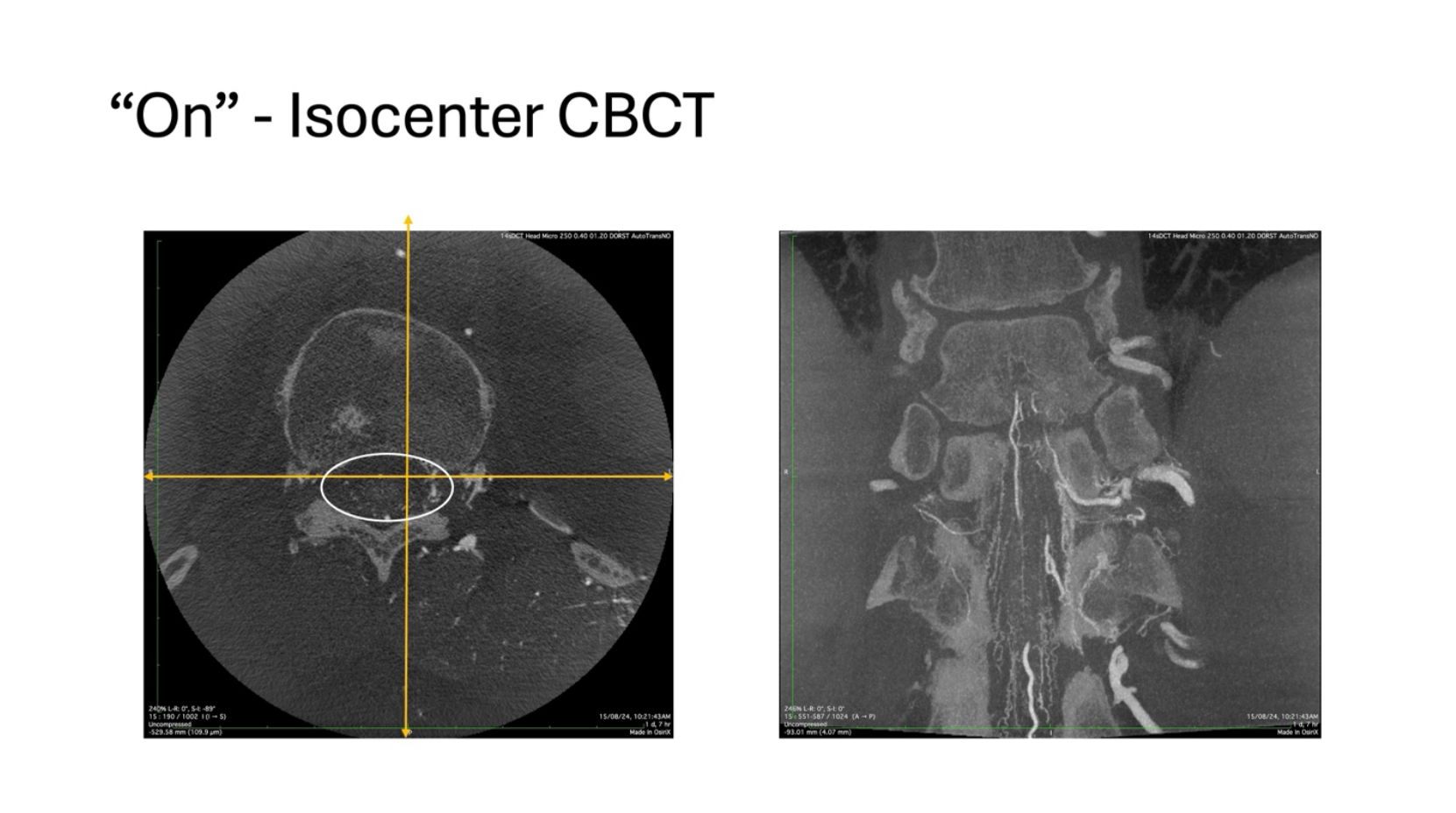
In this exploration, it can be seen that the spinal canal is well within the cross-hairs and the resultant image on the right hand side panel is far more informative that the previous example. The following images will compare them side by side and then the differences will be much more appreciable.


In the images on the right-hand side, with the so called “On” isocenter exploration, it can be very well appreciated that the anterior radiculomedullary branch ascends anteriorly and superiorly to reach the ASA axis. At the same time the radiculomeningeal branch hooks over the ligamentum denticulatum, and travels posteriorly, in a completely different plane to reach the dura at the Dorso-lateral aspect and supply the fistula. With this clarity, the subsequent embolization becomes very safe and effective.
Let us make things interesting – addition of contrast to the equation
The previous sections (except the clinical vignette) dealt with the principles of image generation in the angio suite. These techniques allow us to generate a CT image of the area of interest. However, it is not enough by itself. We need to selectively opacify structures, meaning arteries, veins and everything in between along with any other parts of the anatomy that we might need in a given case. In case of neurological Angio exploration, the contrast may be introduced directly in the arteries, in the veins, in lesions like tumors by direct puncture, or in the capillary bed by using the circulation itself. Based on the contrast introduction, various kinds of images can be generated. Let us see these in a bit more detail. The general principles come first and then we illustrate further with examples.

In this illustration, from the left to right, there are three corresponding images of the same subject. On the extreme left, the CT exploration has been done without the addition of any contrast. Typically, whenever doing a 3D exploration of the vasculature, the first step is to acquire this image which acts as a mask. This is the first spin around the patient.
Following the acquisition of the mask image, contrast is introduced into the vasculature and another spin is acquired. That is represented by the middle image in the panel shown above and this image contains all the information acquired by the mask plus the opacities introduced by contrast injection into the area of interest. In this case the contrast has been introduced into the internal carotid artery and what are seen as white dots in the middle panel are the branches of the ICA that have been opacified. This image can be called the contrast image for understanding purposes as it shows all the structures in the field of view that are radio opaque. This phase marks the end of the data acquisition, and we now move towards the post-processing of all the information that has been acquired.
The third image on the right-hand side of the panel shows what is called as the subtracted image. This is a mathematical process wherein all the data created in the mask is subtracted from all the data acquired in the contrast, meaning all the densities that are apart from the contrast that has been imaged. This leaves behind the subtracted dataset that shows only those areas that have been selectively opacified by the contrast injection.
Mask (M)– the first image of the FOV created without any external contrast introduction.
Contrast (C) – the image acquired after the introduction of contrast.
Subtracted (S) – a mathematically generated dataset with only the extrinsicslly introduced contrast.
Therefore, S = C – M
It is also important to understand that during mathematical manipulations, the nature of the acquired dataset also changes, so in terms of anatomical representation accuracy, the subtracted images are of the lowest confidence levels, even though they look the most appealing to the eye. This is extremely important — pretty much all arterial high-end cone beam images of the best detail are Contrast (or “natural fill”) types.
After this discussion on the concepts of image acquisition and image generation, let us use the vaery same example shown above to create 3D Virtual Reality (VR) images from the same source data and try to understand how things look.

These three images have been reconstructed from the three corresponding datasets used in the preceding discussion. The first image on the left of the panel shows a VR rendering of the mask. Essentially it is just like any 3D reconstruction, and this is used to give information of the bony landmarks, presence of implants like clips, coils, devices, etc. On its own, it is not very informative but in certain situations gives very useful and actionable information, we will give appropriate examples in the later parts of the discussion.
The central panel shows the entire dataset acquired with the introduction of contrast material into the arterial system, the ICA. Even though the vessels are seen clearly, the presence of bony densities are obscuring the finer details of the vasculature. To circumvent this problem, we now move to the third image on the extreme right-hand side of the panel which is the so-called subtracted image. This, as discussed earlier, is a mathematically generated subtraction of the mask from the contrast. The advantage of this image is the extreme clarity seen in the Willisian and immediate Supra Willisian arterial structures, at the same time, the disadvantage is the loss of details in the finer parts of the vasculature, both as a result of the spilling-over of the subtraction, and the lack of opacification of the very distal vessels due to the timing of contrast introduction.
Depending upon the timing of contrast introduction into the system, the arteries or the venous system can be selectively opacified to produce high-definition VR images of the desired structures. For example, if the position of the catheter is in the Internal Carotid Artery, a delay of 1.5 to 2 seconds is used to selectively opacify the arterial system. Of course, this is also dependent on the internal milieu and the hemodynamic conditions at the time of injection. If the circulation is slow and the systolic pressures are low, the delay needs to be increased for the contrast to have enough time to opacify the desired structures.
On the contrary, if the desired area to be explored is the venous system in the brain, allowance will have to be made for the transit time through the capillary bed. A situation will have to be created where the injection is done in the artery, time is allowed for this contrast to clear from the arterio-capillary bed and opacify the venous system. Typically, dependent on the hemodynamics, this takes 8-12 seconds for useful images of the venous system to be created with an arterial injection. Of course, the larger venous sinuses can be opacified directly and 3D acquisitions done.
More information on venous phase imaging is available in the Venous section of a meningioma case

All this discussion is about the subtracted 3D visualization technique. As we have learned, apart from the obvious advantages of this modality, there are pitfalls as well. The mathematical subtraction and the 3D reconstruction algorithms are not perfect and in the process, they tend to subtract unintended data and manage to introduce information that is not actually present!. Also, these are mandatorily binned, so at the very least, 50% of the data is lost in translation.
To refine this technique and circumvent some of the pitfalls, these days we use an extension of this technique that is an unsubtracted, unbinned data set with contrast and this technique is referred to as “High Resolution, Unsubtracted, Unbinned Catheter Cone Beam CT Angiography” a real mouthful. Let us try and understand this technique in the following section.
What is “High Resolution, Unsubtracted, Unbinned Catheter Cone Beam CT Angiography”
The principles of acquisition remain the same. Since this is an unsubtracted technique, only one rotation is done with contrast introduction and the entire data set is reconstructed without binning. Although this sounds simple, the hardware limitations for this technique are massive. The acquisition and the contrast injection are straightforward. The problem comes in managing the massive amounts of data that are generated. Imagine our flat panel detector has 2584×1904 = ~ 5 million pixels. Now all the data needs to be shu led from the detector to the machine, then reconstructed quickly, rendered etc. for this, the hardware must have a huge bandwidth and memory. There are two prospective solutions to this problem. Either you install a super-computer in the Angio suite (not practical) or you reduce the amount of data to be processed. Since the conventional techniques of reducing the data by binning are not tenable, the only other solution if to reduce the area of the detector that is used to capture the image, and this results in a relatively smaller FOV for these studies. Typically, most modern machines allow a 10×10 cm FOV for these ultra-high resolution studies, and we will see the same with examples.
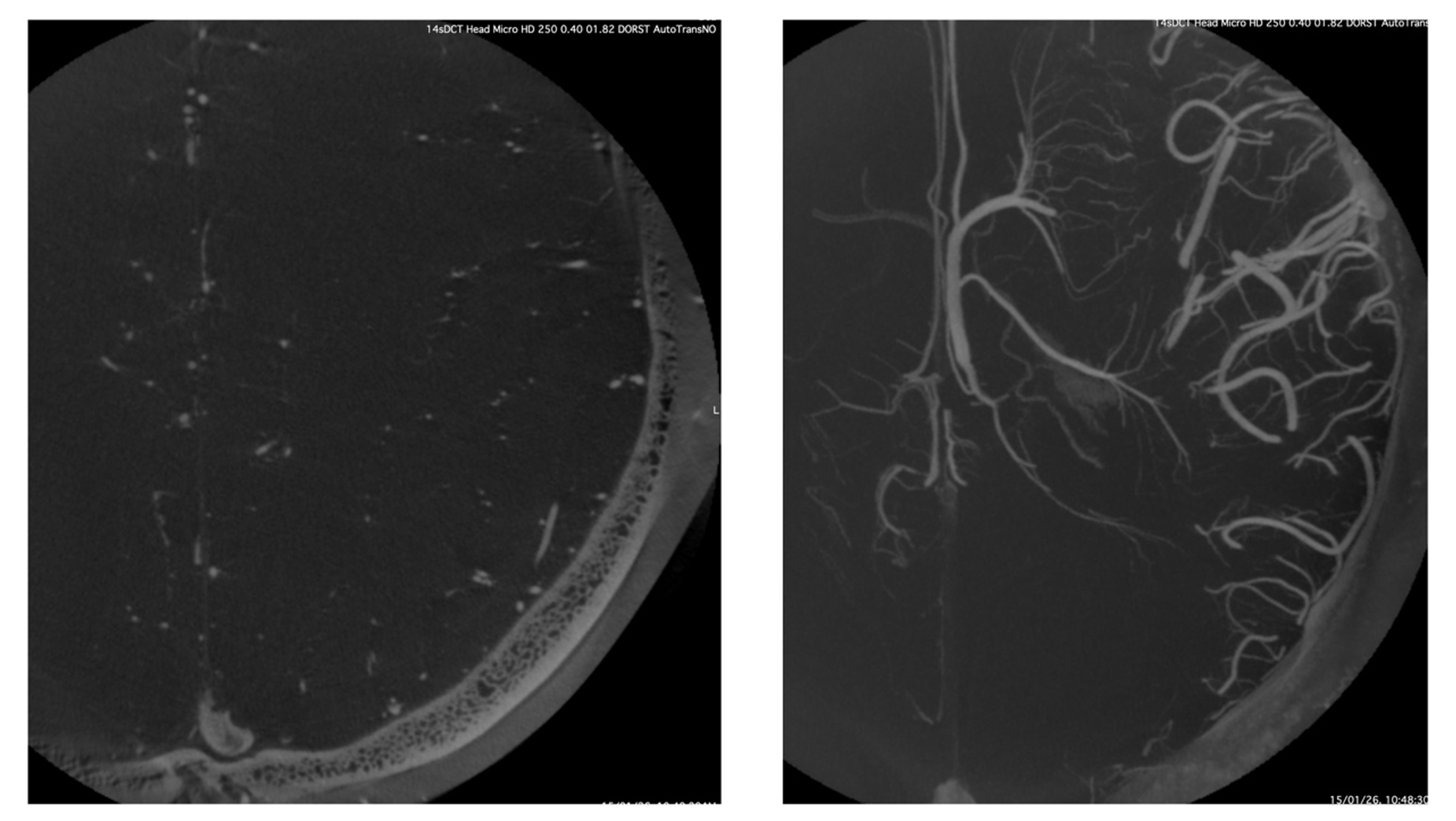
This example shows the typically smaller FOV that is explored by this technique. One can appreciate the unsubtracted source axial image with the smaller vessels seen very well in the depths of the white mater, although only half of the hemisphere is fitting into the FOV. The right-hand panel shows the MIP reconstruction of the same source image showing the massive details of the deep venous system in exquisite detail. One basic principle of this technique is a complete opacification of the arterio-capillary-venous system throughout the rotation to ensure uniformity in the imaging. Therefore, this technique does not have temporal resolution, i.e., it is not able to tell us what is artery and what is vein, but the spatial resolution is massive.
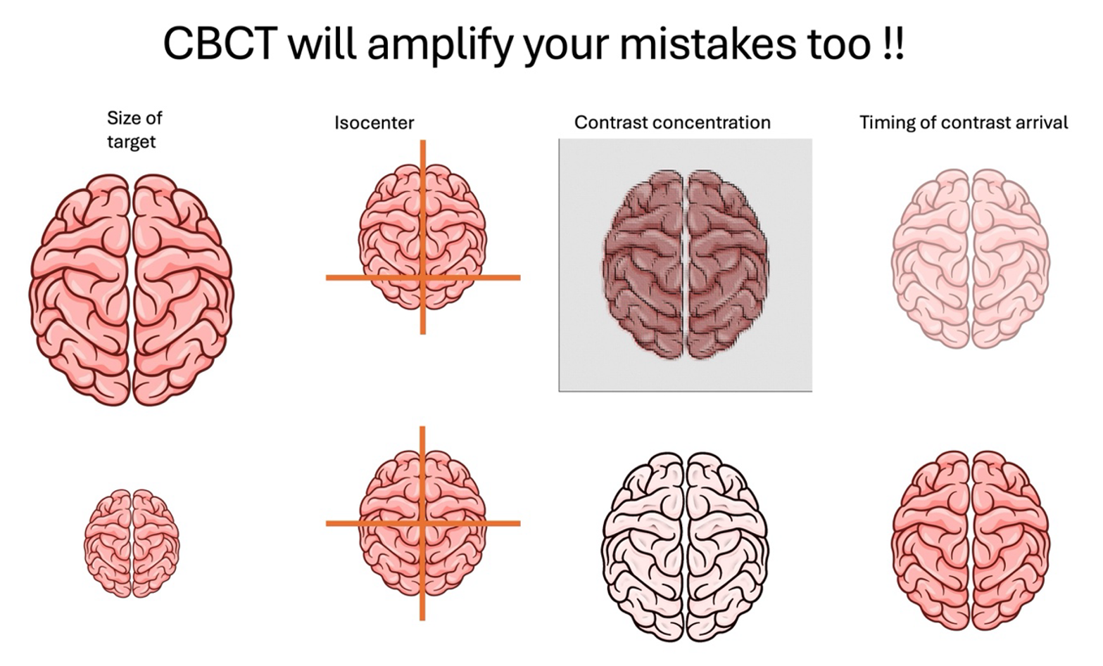
The variables in “High Resolution, Unsubtracted, Unbinned Catheter Cone Beam CT Angiography” – timing, contrast concentration and movement – or the lack of it
Injection of contrast into an artery and following a pre-specified delay, a 3D acquisition with a small FOV is the basic tenet of this technique. As has already been mentioned, we aim to opacify the entire vascular tree with contrast and then start the rotation for a complete visualization of the entire system. Typically, under standard hemodynamic conditions, the trans cerebral transit time is 6-8 seconds. Therefore, from the point of injection, the rotation must start after a 6-8 second delay to make sure that the entire tree is filled with contrast. Depending on the machine being used, the rotation speed can be anywhere from 10-40 degrees per second, and thus the rotation times vary between 7-15 seconds. Taking these timings into account, the delay must be 7 seconds and the total injectioin times including these 7 seconds must be 14-21 seconds. With this protocol we can derive the best possible images, and we will illustrate the e ects of all these in a moment.
Contrast concentration
Usage of undiluted contrast for these high resolution CBCT images should be a no brainer. However, that is not the case. Some more physics. We briefly touched upon this topic earlier but now let us dive into it again. Let us start with an example.
The following image is from a patient who underwent the exploration of the posterior fossa with inadvertently 100 % contrast being injected during the study. Although the images were showing good opacification, a closer inspection shoed multiple streak artifacts and also loss of detail in the finer parts of the vasculature like the perforating arteries of the brainstem.
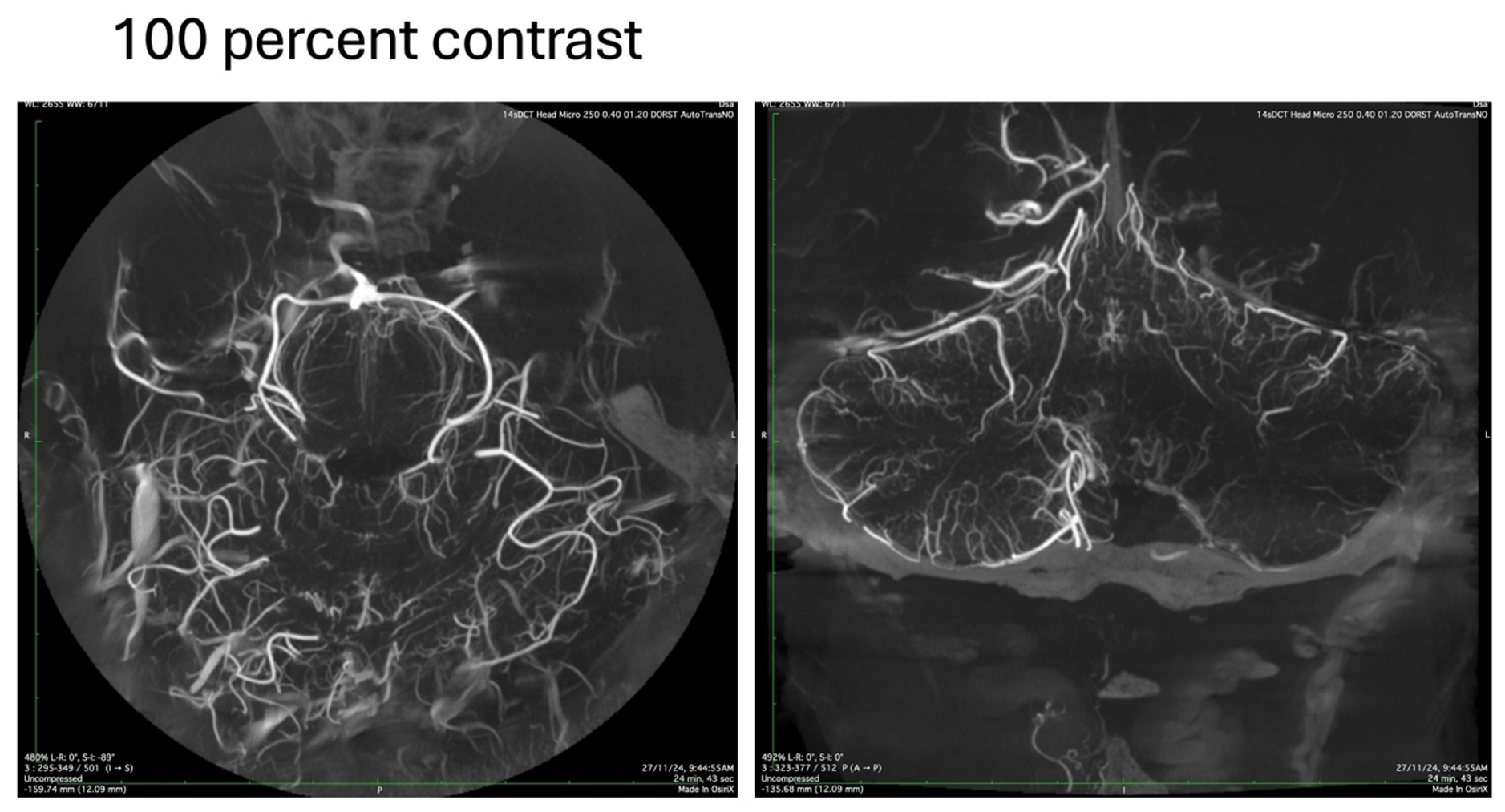
This happens mainly due to a phenomenon known as “beam hardening”. What this means is that when an X-Ray beam hits an object of high density like the petrous bone, teeth or undiluted contrast as in this case, the components with the lower frequencies get absorbed or reflected. Only the high frequency components that have more penetrating power make it through to the detector. These “Hard” beams produce viable images of the opaquer structures but at the same time are too strong and go completely through the smaller vessels which have less amounts of contrast in them, thereby losing the finer details. Let us see the same example when the study was repeated with a diluted contrast.
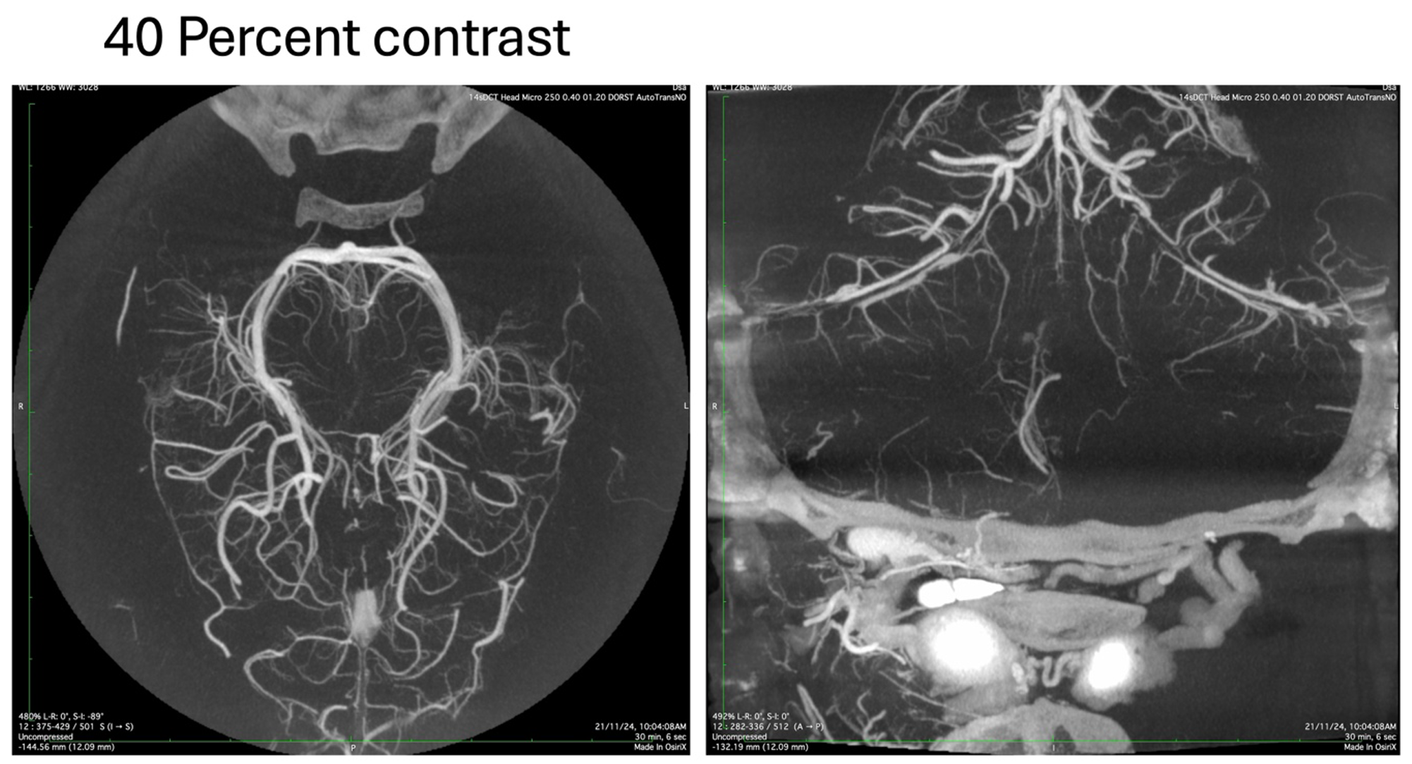
The image acquired with the diluted contrast is more homogenous without any streaking or loss of details in the finer vessels. By trial and error, we have been able to determine that the optimum contrast strength is between 35-50 percent, depending on the pathology being imaged, the hemodynamics and the area of interest.
Overall, there is no single contrast concentration that is best for everything. When learning to do this, or for those that are not particular about imaging, the tendency is to stick to whatever concentration someone else told you to do. That is a mistake. Volume Rendered images, for example, generally do better with higher concentration (the smaller vessels are not as well seen there anyway, while the larger ones do better with more contrast). If however MIP images are what is needed primarily, then lower is generally the way to go. Any master of anything knows that all details are important, and how to change them to optimize the image for the clinical question at hand
Movement
The 3D images that are generated by a CT scanner of any time is dependent on a very basic principle. During the acquisition, the relationship between the detector and the object being imaged has to remain constant in all the 3 Axes, throughout the length of the acquisition. Any change in the relative position of the object-detector relationship will result in a skewed reconstruction and these are seen as artifacts on the final image. In subtracted 3D formats, different vendors have algorithms that reduce the e ect of these movements, but as we move towards higher resolutions with smaller FOV’s, even respiratory movements and cardiac pulsations are enough to introduce noise into the final rendering. Let us see an example.
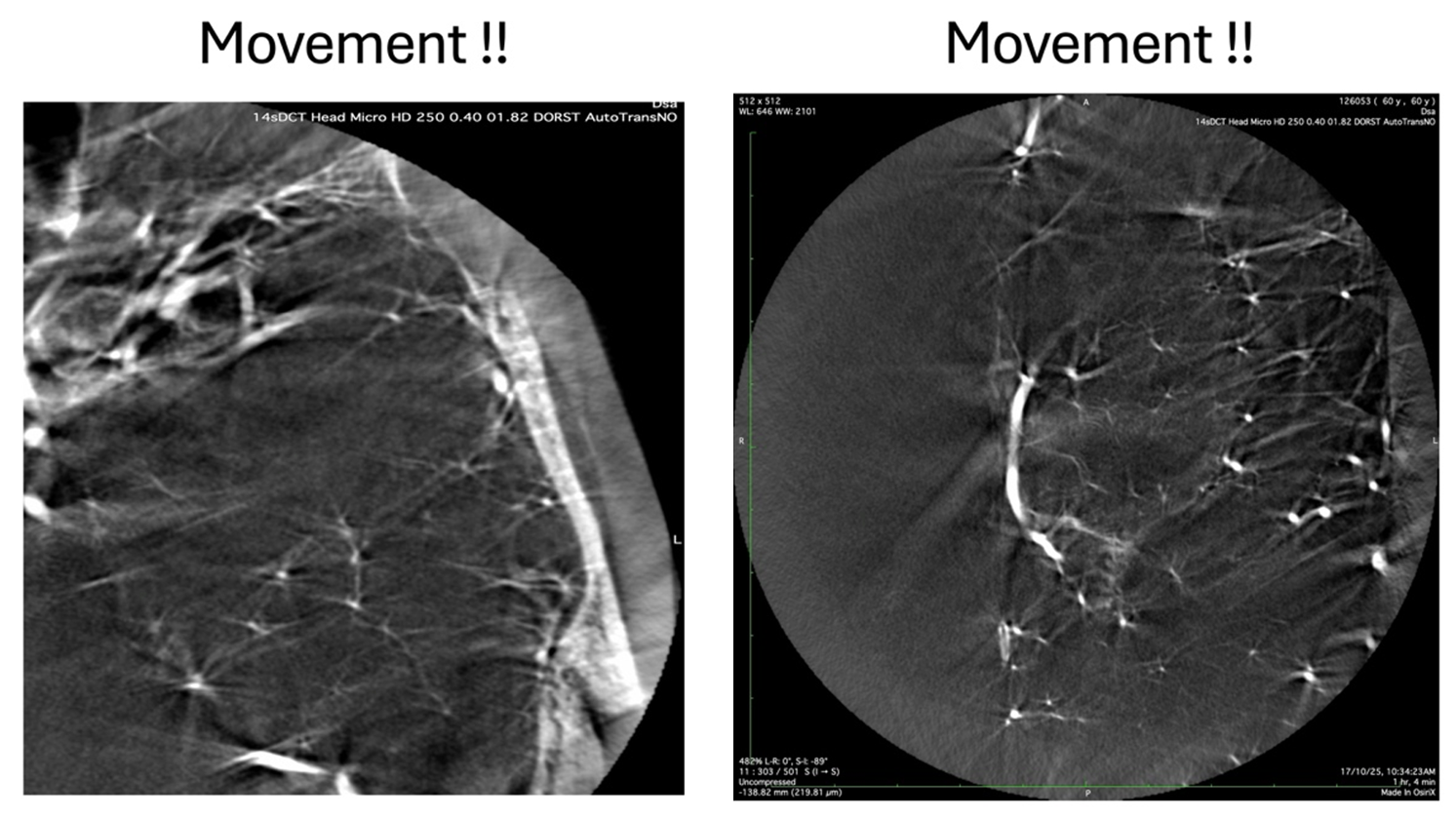
This example shows the results of patient head movement due to respiratory motion on the f inal rendition of the vascular anatomy. Therefore, it is imperative to minimize all these motions by having the patient under GA with apnea during the acquisition. Proper fixation of the head on the head holder is a prerequisite. Whenever GA is not feasible, a conscious patient can be given appropriate instructions, but it becomes a real challenge with uncooperative patients. The same types of artefacts can be seen if the detector is not calibrated properly and moves in multiple plains, just to the tune of millimeters, during the acquisition.
Summary of Principles
1) the area of interest needs to be pre-determined and the FOV needs to be as small as possible for each manufacturer and specific machine
2) the area of interest needs to be positioned in the isocenter of the C-Arm, both in the AP and the lateral planes
3) for High Resolution CBCT exploration, typically diluted contrast material is used to reduce beam hardening, streak artifacts and loss of details in the small vessels, typically 30-50 percent
4) the entire vascular tree has to be saturated with diluted contrast, which favors longer delays, and a total injection time of 14-21 seconds depending on the equipment